
Janssens, Chow & Nieuwdorp - Turning DataFrames into Pretty Pictures with Plotnine | PyData NYC 2024
www.pydata.org Learn how Plotnine, a Python package inspired by R's ggplot2, enables the creation of sophisticated and effective data visualizations with minimal effort. This tutorial will explain how Plotnine's grammar of graphics approach provides a flexible, intuitive way to visualize data, either as ad-hoc plots or fine-tuned graphs suited for communication. Quick links Presentation: https://bit.ly/plotnine-tutorial GitHub repository: https://bit.ly/plotnine-repo Slideshow about what to expect: https://bit.ly/expect-plotnine PyData is an educational program of NumFOCUS, a 501(c)3 non-profit organization in the United States. PyData provides a forum for the international community of users and developers of data analysis tools to share ideas and learn from each other. The global PyData network promotes discussion of best practices, new approaches, and emerging technologies for data management, processing, analytics, and visualization. PyData communities approach data science using many languages, including (but not limited to) Python, Julia, and R. PyData conferences aim to be accessible and community-driven, with novice to advanced level presentations. PyData tutorials and talks bring attendees the latest project features along with cutting-edge use cases. 00:00 Welcome! 00:10 Help us add time stamps or captions to this video! See the description for details. Want to help add timestamps to our YouTube videos to help with discoverability? Find out more here: https://github.com/numfocus/YouTubeVideoTimestamps
image: thumbnail.jpg
Transcript#
This transcript was generated automatically and may contain errors.
Hi everyone, so this is the final workshop of the first day of PyData conference and thank you for sticking with us so long. We are gathered here today to attend the workshop of Thijs, Michael and Jeroen. They talk more about visualization and plotnine but so yeah, so thank you so much for coming here all three of you and we're excited.
Thank you. Yeah, thank you for the introduction and thanks to you for joining us today at this plotnine tutorial. In the next hour and a half, I won't be able to cover everything there is to learn about this wonderful data visualization package but at least I'll be able to cover the most essential concepts and provide you with a toolbox that you can use so that after this tutorial you'll be able to produce data visualizations based on your own data using plotnine.
So I'm very excited. I've been using this package for a long time already and it seems that it doesn't really get the attention it deserves. So again, I'm really happy that you took this chance to learn more about it.
My name is Jeroen and I am accompanied today by two lovely assistants, Thijs and Michael. So if you have any questions regarding your setup in the beginning or later on as we do the exercises then yeah, you can ask them for help. If there is anything in general, then please ask away as well. I really encourage you to ask questions. I have more than enough material for this hour and a half but I think it would be just so much more fun if you also would ask questions.
Overview of the tutorial
So for today, what I have in mind is let's first establish that you're at the right tutorial right now or that you're watching the right YouTube video. So I'll be showing you some examples of what you can create using plotnine. Then a little bit about the importance of data visualizations. It's all too often that I see people working with data and never take the opportunity to actually look what's inside there. They immediately go from raw data to clean data and then machine learning model.
So plotnine in a nutshell, what are some of its basic features, the concepts that you need to understand because there is a learning curve associated with plotnine. But once you do have that dialed in, then you'll be able to produce beautiful data visualizations. I'll also provide you with resources that you can use not only for the exercises in this tutorial but also afterwards when you want to visualize your own data. And then as a bonus, we have Michael to talk a little bit about the package that he has co-created, Great Tables, which is also a form of data visualization but then still different enough to warrant a separate package.
All right, so I do encourage you to follow along and to do the exercises for this. You of course need to set up everything. You can go to the GitHub repository that we've set up to scan this QR code. There's also a link in the description on the PyData website. And then you have two options. You can either use Posit Cloud or you set up things locally. We've provided instructions to use UV, but if you have a different method of installing things, then that's of course fine. The two main packages that we'll be using today are of course plotnine and then also a little bit of Polars to do some light data wrangling.
Examples of what plotnine can create
So is this tutorial right for you? Let me show you a couple of examples, a couple of data visualizations that have been created using plotnine. Here's a set area chart. Here's an annotated scatterplot. It doesn't always have to be this fancy. This is a heat map that I pulled from plotnine's documentation. Here's a line graph where we highlight the Polars package. These are the number of GitHub stars that these packages have amassed over time.
And now is actually also a good time to do some advertising because Thijs and I, we are very close to finishing our book, Python Polars, the Definitive Guide, which should come out February next year. And in that book, there are also some visualizations. One of them is this based on data from Citibike. And that's actually also the same data that you'll be using during the exercises.
Here's an animation. We're applying some dimensionality reduction on a high dimensional data set. What really matters is that it's an animation created using plotnine. And here's an example of a great table using Great Tables.
Why data visualization matters
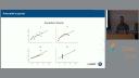
Maybe you're already convinced. For those who have not yet seen this data set, these are four data sets, each consisting of 11 data points. And if you were to compute some basic descriptive statistics, you'll find here on the right that they all have the same values. And then you might be inclined, well, these are the same data sets, until you actually visualize them. These are four different data sets. And this data visualization, you guessed it, has been created using plotnine.
And so this is, I believe, the best argument for why it's important to visualize your data. And only that way, you could really get some insights into the underlying structure.
And so this is, I believe, the best argument for why it's important to visualize your data. And only that way, you could really get some insights into the underlying structure.
And this is the corresponding code that you would need in order to create this data visualization. And this is quite large. I can imagine that this is quite overwhelming, quite intimidating. It's quite a lot of code. Lots of functions in there that you've not seen before. You may guess a couple of things, what each function is trying to do.
But what I hope to achieve in this tutorial is that you'll be able to look at this code and say, OK, I know what's going on. And not only that, that you're also able to come up with this yourself. And so it's also good to know that I didn't start with this. Of course, when you're developing software, you never just type it out in one go, right? This is an iterative process. So what you see here is almost that same data visualization, but then only the ascensions. So this is created using only four lines of code. Now that's a lot less, right? That's comforting to know. And that's one of the strengths of plotnine is that you can easily create these ad hoc data visualizations fairly quickly. And then once you have that, you can iterate on that and then refine your visualization, make it ready for publication.
What is plotnine?
All right, so what is this plotnine? Well, it's a Python package created by Hasan Kibriye. He now works at Posit. And it's based on an R package called ggplot2, created by Hadley Wickham a long time ago. So plotnine is stable. I've been using it for at least five years. But it's just not as complete yet. And it doesn't have the same ecosystem of plugins that ggplot2 has. Still, I'm certain that you'll be able to create about 95% of all the visualizations that you do want to create.
There are some subtle syntax differences between ggplot2 and plotnine because, well, one is an R package and the other is a Python package, right? And these languages, they're not the same. So still, the API is very consistent. So we can use a lot of the resources that have been created for ggplot2. ggplot2 has been around for over 12 years. We have cheat sheets, we have a gazillion blog posts, plenty of examples. And with just a few tricks, we can actually use all that for our own purposes when we're creating a visualization using Python and plotnine.
The grammar of graphics
So here are some of the concepts that I think are important for you to grasp. Like I said, there is a learning curve. It will take some time, but there's a reason for that. The name ggplot, or the two g's, they don't stand for good game. They stand for the grammar of graphics. And this implies that there is some structure to this, some grammar. You see, all these examples that I've shown you in the beginning, they look very different, but they actually have, well, they've been built using the same grammar. They share a lot of structure to them. There's a certain language to create this.
Okay, we'll go over each of these concepts one by one. And I also have some exercises to see if it all sticks, so you can apply those concepts to that city bike data. And here's the first one. Your data. Your data can come in in various formats. And generally speaking, you want your data to be in a tidy format. Now, I don't have time now to cover what that means, but in practice, it's usually a long data frame is good, and a wide data frame is bad.
Yeah? So you can imagine that those 44 data points of the Anscombe Quartet can be represented in multiple ways. On the left, we have a long representation, where each row is one data point. And on the right, we have, well, we only have 11 rows. And then we have, well, we need more columns, because the data sets, right, these four data sets there may not be next to each other. The long representation is good, because what plotnine does, it will turn every row into a thing that appears in your data visualization. This is known as a geometry.
So once you have your data, you can start creating a data visualization. Now, the package is called plotnine, right? I think I've told you that. But the function that you need to use in order to get started is still called ggplot. Yeah? Don't ask me why. But I think, well, if you do want, let's say you did want to ask me why. I think it is because Hassan really wanted to be consistent with ggplot2's API, right? So ggplot.
Here, we specify two arguments. First one is the data frame. And this can be a Polars data frame, but it can also be a pandas data frame, right? Under the hood, it is still being converted to a pandas data frame. But all this to say that you don't really need to know Polars in order to use plotnine. It is, of course, helpful if you are able to do some data wrangling in Python using a data frame library.
So first argument is the data frame. And this second argument, it may look a little bit strange at first. We use this AES function, which is short for aesthetics. And what we do here is we map the columns that we have in our data to aesthetics, right? You can view aesthetics as properties of the geometry that you're about to use. So you can imagine that in this case, we're using a point. Function geom point will create a new layer that creates a point for every row in your data frame. Now, what are the essential aesthetics or properties of a point? Well, it should have a location, right? X and Y.
You can leave out those two arguments. If you want to map any additional columns to additional aesthetics, then you need to specify them. For example, if you want to change the color of each point. But this is the essence of plotnine. You get some data, you specify which columns should map onto which aesthetics, and then you specify geometry. In this case, we're creating a scatterplot using the geom point function, but it could also have been a line graph, a box plot, an area chart, you name it.
Q&A: aesthetics, imports, and setup
So I see that aesthetics, that function is being used in several places. What are the expected arguments inside to be brought as a function? Aesthetic is one of the arguments, and then I thought, you can go to the previous slide. In your previous example, inside your point also, you can have an aesthetic function argument.
Alright, so to summarize your question, we see here in this example that the function AES is used multiple times. It's used as part of the ggplot function, where we're starting a new data visualization, but then also inside the geom point function. And what the short of it is, is that you can override or expand on the mapping that you do. Alright, so essentially if you combine these two AES methods together, you'd say what you get is that the x aesthetic, x value, is based on this one, the displacement column. Y is based on the hwy highway column, and the color of each point is based on the class column of each row. And the reason we're specifying it here on the geom point level is because we only want to influence those points. We don't want to influence that line that we see down there, which is created using the geom smooth function. It's a very good question, and it's actually my bad that I've already introduced this in the beginning, because this is one of the concepts that I will cover later on.
So, do you want it to use from plotnine import star, or sometimes you try to not do that? Yeah, alright. Fantastic question. The question was, I see here, from plotnine import star. What's up with that? Okay, you didn't phrase it like that, but I can imagine that a lot of people are thinking, okay, this is just not done. And I agree, right? When you're developing software, you want your namespace to be clean, right? When you import things like this, everything gets in your little namespace, and that's not a good practice. And for software, I agree with that. When you're working inside a notebook, and you are experimenting, you're experiencing ad hoc data visualizations, this is my preferred method of importing everything from plotnine, because then it's just a lot less typing. It feels more like the R way of working, and that's what I used to do in another life. But if you do want to import plotnine neatly, then what is often done is that plotnine gets imported as P9. Just like Polars often gets imported as PL, or NumPy gets imported as NP, the convention for importing plotnine then would be P9.
Statistical transformations
Okay, the third concept. So there are certain statistical transformations that you can do using plotnine. Think about grouping or counting things. This is quite convenient. So what I'm doing right here is I'm using the function geom histogram. And what's interesting to note is that I am not explicitly specifying this count column.
Can we just appreciate for a second how many things plotnine does for you out of the box? You've got your limits all set up based on the data. You've got your labels. You've got default colors. And so lots of legend. Lots of sensible defaults. And it is good to know that each of these can be overwritten. You want the colors to be different. You want the font to be different. Everything. But right now we're still creating these quick data visualizations. So with geom histogram, it's a bunch of bars. But what is happening under the hood is that there's also some counting going on. And so plotnine creates this new column for us, count, which gets mapped to the y-aesthetic.
So it's a bit confusing, but notice that the y-column is actually mapped to the x-aesthetic. Just to make things more confusing. So this is conceptually what is going on under the hood. You provide it with a data frame, but before plotnine actually visualizes everything, it furnishes us some, in this case, a group-by operation. And this is optional. When all the data that you're using for visualization is already in the data frame, then this is optional. And you are still free to do any of these aggregations yourself.
Scales
Alright, yet another concept for plotnine. And this one, this is a tricky one. So bear with me. For each aesthetic mapping, I should say, there's this translation going on from values in your data frame to something that appears in your data visualization. And there's almost never a one-to-one relationship. Somehow, plotnine has to convert those raw values into pixels. So that's what this mapping is all about. And this is influenced by many things.
So, relatively speaking, when the x value in a data frame related to a certain row is higher, the corresponding point in the data visualization moves to the right. But by how much? That's determined by a number of things. First of all, it's determined by, well, where do we start this x-axis? Does it start at zero? And what is the end? And is it linear? Or is it on a log scale?
So, this can be influenced using a collection of functions that start with the word scale. And there is a scale for every aesthetic out there. So in this particular example, what I've done is I have turned the x-axis into a log scale. Using the function scale underscore x underscore log 10. And for the y-axis, well, I kept the type of scale, which is by default, there's always a default, and for x and y scales continuous, I changed the limits. So, by default, those limits are based on the data, on the lowest value and on the highest value, and then some. But you can apply those. So here, I said, okay, now, I absolutely want my y-axis to start at zero and to end at 20.
But scales go beyond the location of a point or of any geometry. Like I said, there is a scale for every aesthetic. There's also color, right? Plotnine has to translate raw data values into some color. And depending on the type of the column and depending on what you want to convey, this can be different.
What I've done here is I've used a different color map. These come from the Brewer collection of palettes, so to speak. So these take some very particular arguments, so the type and the palette. And what you're doing here, then, is you override the colors that are being used for data sets. This is, of course, a discrete column, the quality of it. But if you have a continuous value, you might only use a gradient.
And also for the size, it's a bit contrived in this example, but it does help me make my point here in that the size of each point is also determined by the values in the Y column. So that's a little bit redundant, because we're already using Y for the Y axis. So what I've done here is I have said, okay, the minimum value that I am going to consider in the raw data that will determine the size of each point is 5. Right, so if the value of Y is below that, it gets the same size. And same thing, the upper limit is 10.
So the points are very, very small here, but you might be able to see that any data point, and there are four of them, that are 10, that have a value of 10 or higher on the Y axis, all have the same size. And the range there, that's the second argument of this scale size continuous function, determines, okay, what is then the actual size being used? So how small should the smallest point be, and how large should the largest point be? So, conceptually speaking, what we're doing here is we're mapping raw data values onto some aesthetic values, and that translation, that's what we're influencing right here.
And this is, I found this at least to be the toughest concept to wrap my head around.
All right. Yeah. So to summarize your question, what's up with that plus sign? And this is, again, this is history, because that's how R's ggplot2 does things. This plus operator has been overloaded, and nowadays, if you're familiar with R and the tidyverse, you use the pipe operator to combine things. And in Python, we're used to do method chaining. But since Hasan wanted to stay close to the original API, he used the plus operator. And indeed, what you said, right? You're adding layers, but only certain functions add layers. So those who start with geom add layers, and there's also, there's a couple of others, but that's outside the scope of this tutorial. But everything else also gets added, but it's not technically a layer that you're then adding. So conceptually, it's like method chaining, only a different syntax, and I know that takes some getting used to. But trust me, you will be able to get used to that, just by using that.
Layers and inheritance
Alright, yet another concept for plotnine. Layers and inheritance. And we already had a question related to this. Remember, we had a question as in, why do I see the AES function being used multiple times? So, first of all, layers. Every geom function creates a new layer. And the order here matters. The one you specify first gets drawn first.
And, the inheritance part here refers to both the data and the aesthetics mapping. These are two things that we can specify in the ggplot function. Our constructor, so to speak. And when you specify them at this top level, then all the layers will inherit both the data and the aesthetics mapping. And this is, for a lot of cases, this is quite convenient. Right? You don't need to specify which data frame you want to use for every layer separately. But you can, if you want to. Sometimes you do want to use a different data frame for another layer. Think about, okay, so, bear with me here, but you have a scatterplot. Right? With a couple of clusters. And you also have some labels. Some text. And you want, at the center of each cluster, to have a single label.
Now, the labels need to come from a separate data frame that only has a few rows. One row per cluster. So you have to do some aggregation. Or maybe even some clustering yourself. But then you are able to add a new layer using geom text, geom label. Right? Add those labels. And say, okay, I don't want you to use the default data set that contains all the data points. I want you to use this other small data frame which just contains the labels and the coordinates where they should be put.
So that's for the data. And then for the aesthetics, same story. Sometimes, not every layer has to have every aesthetics mapping. Coming back again to labels. Right? For a label, you need to specify, okay, in which column do we have the text? Right? And that's always specific, that's very specific for all the geometries, text and labels. So, what I usually do is I reuse the AES function and only add that specific mapping.
Something that I haven't really included in this presentation, but I do want to point it out, is this facet wrap function. I've already shown it a couple of times, but I've never really, you know, explained it to you. Well, what this does, it creates facets. It creates these four panels, one for each data set, one for each unique value in the data set column, which is all the Roman numerals one through four. And, I think this is, this really captures the idea that you use plotnine in a declarative way. Right? You're not programming this procedurally or anything. You specify what you want to visualize, and then plotnine will figure out how to do it.
Static aesthetics
So, we've talked about these aesthetics, right? Properties that influence how a geometry is being drawn. Most of the time, we want these to be based on our data, right? Because we're creating data visualizations. Sometimes you want things to be static. You want to set a certain aesthetic to a particular value. And the best term that I've been able to come up with, is that they're aesthetic-aesthetic. Which, for example here, all the points have the same color. This is not based on data. Usually, these are things that you tweak.
And the names for the aesthetics remain the same. Color, fill, even x and y, but then you would have everything at the same location. That's usually not very helpful. But, if you want to do this, then make sure that these keyword-argument pairs, such as fill equals dark orange, and color equals sienna, and size is three. Okay, so we have here three static aesthetics in a row. Make sure that they're not part of the AES function. Yeah, that's a common pitfall. However, when an aesthetic has to be based on data, it needs to go inside the AES function. Otherwise, you'll get an error.
Great Tables
Alright, thanks Jeroen. Okay, so tables. I'm a giant fan of plotnine and more recently I've been working on a sort of related area which is kind of like the step-cousin to a plot, a table. They're both a form of data visualization but it always seems like tables are a little bit different, a little bit funkier, so I'm excited to get into this.
So here's, this is what I mean by, I'll call this a display table, so this is a table that you might want to present for publication. And notice that here we have a lot of elements you'll find in plots, so like the background's color, we actually have a small plot embedded in the table, we have a lot of text information, percentages, things like that. So this could, parts of this could be in a plot, but I think the key to tables and what distinguishes them from plots often is that there are a couple things.
So one, a plot usually has only a few dimensions, so you use a few columns and you might have an x and y axis, you might have some color, but you're limited to a few dimensions. Notice that tables, your values are often shown as columns, so you don't have to have just an x or a y, you could actually show 5 or 10 different measures side by side. So that's an important use case for a table where plots tend to not work as well. The other really valuable use case of a table is that they often encode the raw numbers or something close to the raw values. Plots, often times, plots are really good at showing you patterns, so they might show two of these in the scatter plot, but it's hard to pull out the raw numbers.
The other really valuable use case of a table is that they often encode the raw numbers or something close to the raw values. Plots, often times, plots are really good at showing you patterns, so they might show two of these in the scatter plot, but it's hard to pull out the raw numbers.
So this is the gist behind a table. Good thing is tables tend to be very compact, so they're really good for metrics or dashboards where people are really interested in the raw numbers, you see this a lot in sports, like basketball or soccer, where you break down athletes and teams.
I'm going to very quickly run through some of the elements of a table. So I'll say there are three key pieces: there's structure, formatting and style. And what I mean by structure is things like a title, so notice that a data frame doesn't have a title on it, so we put one over this table so people can get the gist of what we're displaying. We have column labels, so we've given nice names to the columns, whereas data frames we tend to do things that are easy to type. And then grouping rows, notice that Manhattan, all rows in Manhattan are grouped together, so this is a way to do a little bit of natural grouping.
For formatting, notice that the percentages here have been cleaned up a little bit, so these are whole numbers, so that's often just to make it a little bit easier to read and pull information out of. The other type of formatting we'll talk about is a data prompt, so we changed, this was essentially a list of data here, and we changed those into small visualizations, so formatted to make it quick to read. The last thing is styling, so we made the background here recolored it, so people can pull out trends, and styling is often very similar to doing things that happen in plots inside of a table, so you can emphasize trends and patterns.
I will note, I noticed that in the Posit Cloud I think it just doesn't have enough resources, it's a little bit under resourced. So what I'm going to do is I'm just going to grab a specific week, so I'm going to grab like 7 parquet files.
So this is doing a little bit of data analysis, prep everything. So here's a data frame, this is kind of the raw data, notice this is like guts out, this is good for when you're analyzing but you wouldn't want to show people this. And here's this list, you can do a nanoplot. And then here's a GT, and here's the final table if you're interested.
The thing I'll note here is the key is all the structure pieces, they often start with tab or cols, so this is for doing something to the table. Formatting, notice these all start with fmt, so it's quick to find all the ways to format. And styling is a little more all over the place, we have this thing called data color, which is meant to really easily fill in the background on the table. And then there's another function called tab style that does a lot of stuff. So that's just to show you the rough structure of Great Tables and the types of tables. So, step cousin to plots, a little bit different and the key is often when you want to access the raw data or really compactly have a lot of measures side by side.
Yeah, you said you use this, do you use this for publications? Yeah, if so how do you copy it from here to, I don't know, Linux? So the website for Great Tables, that's a website, we use a tool called Quarto, if you go to quarto.org. It's similar to like how you would render a notebook, you can render it to like an html or a pdf or to the other types. So we often use this, this is what the Great Tables website is made in, just because it makes it easier to produce, but you could use whatever you use to render a notebook.
Wrapping up
Thank you Michael. I'm a big fan of Great Tables. Thijs and I, we are actually dedicating a section to Great Tables in our upcoming book. So hey, let's just wrap up this tutorial here because we are close to an hour and a half.
You've been a great audience. I walked around, everybody was doing the exercises, lots of great questions. And I feel that I have been able to really cover a lot of ground here. Not everything yet. I skipped over the fascinating part, theming. That's when you really make the step from ad hoc to publication ready visualizations.
My recommendation then is if you're interested in this, try it out as soon as possible. And then also look into the feed, there are plenty of resources at the end of this presentation for you to continue your learnings. I'm going to be around and so is Thijs and Michael for the rest of this conference if you want to chat about anything. One more plug, Thijs and I are also giving a talk on Friday about how we converted a large codebase from pandas to Polars, in which you will learn more about Polars specifically, which we've used of course a little bit in some data wrangling.
Is it vectorized? Well, it uses matplotlib underneath it, it's rasterized, although matplotlib does have other rendering attributes, you can do SVG, but it's not interactive. That's perhaps the only downside, sometimes depending on what you want to do, you want to be able to interact, you want to be able to zoom and pan, select things. If that's what you want, there are other packages out there, Altair, or probably static ones.


