
Lightning Talk | Andreas Hofheinz | leafdown: Interactive Multi-layer maps in Shiny apps
Interactive maps are indispensable tools for exploring spatial datasets because of their real-world context and intuitiveness. For a comprehensive understanding of the data, it is often necessary to switch between several map layers (such as states and counties) and to analyze multiple variables simultaneously - both of which are challenging. In this talk, I will show how we can overcome these challenges using the leafdown package, which allows us to create multi-layer maps embedded in Shiny apps. Talk materials are available at https://github.com/rstudio/rstudio-conf/blob/master/2022/andreashofheinz/leafdown_presentation%20-%20Andreas%20H.pdf Session: Lightning Talks
image: thumbnail.jpg
Transcript#
This transcript was generated automatically and may contain errors.
Hello everyone, my name is Andreas Hofheinz and today I'm going to talk about interactive multi-layer maps in Shiny with the leafdown package. For my talk, I'm going to use the Meteostat weathers record keeper dataset, which contains monthly measurements from over 2000 weather stations in the United States, which measure variables such as the average temperature and precipitation. And the question I want to discuss in my talk is, how can we most effectively explore this data using insights into how to solve common problems and overcome the limitations of simple maps.
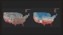
When we work with spatial data, well, it is usually helpful to visualize the data on a map because of the geographical context and the intuitiveness that comes with it. So in this example, we see the average temperature per state and already at the first glance it becomes clear that the average temperature in the South is higher than it is in the North. However, one phenomenon we often observe when we aggregate data at higher levels, such as the state level, is these heartbreaks at the borders. Here it looks like everywhere in California the average temperature is quite high and as soon as you take a single step into Oregon, the average temperature drops significantly, which is probably not the case, right?
But the question is, how can we explore this in more detail, or in other words, how can we zoom in? And one way to do this is to trail down to see the data at a more detailed level, in this case at the county level. In this visualization, we see that there is indeed no heartbreaks at the state borders, but rather a smooth transition and that the overall high average temperature of California is primarily caused by the hot South.
So you might wonder why we don't aggregate the data directly then at the county level and why do we even bother to aggregate it at the state level in the first place? Well, let's have a look at what happens when we plot the average temperature for all the counties at once. In my opinion, this looks quite cluttered and the overall temperature trend is not that easy to see, especially when we compare it to the state aggregation map from before. I'd argue that it is much easier to see on the right-hand side that the average temperature in the South is higher than it is in the North. And this is one reason why it is really important in many spatial data analysis to switch between several aggregation layers to be able to analyze both the overall trends as well as more regional trends.
And this is one reason why it is really important in many spatial data analysis to switch between several aggregation layers to be able to analyze both the overall trends as well as more regional trends.
Visualizing multiple variables with Shiny
Okay, let's return to our map showing the average temperature per county. Often, we are interested not only in one variable at the given point in time, but in multiple variables and their relationship or their development over time. So another question is, how can we visualize multiple variables simultaneously using a map?
And one approach to do this is to embed the map in a Shiny dashboard and connect it to other dashboard elements like charts or tables. By selecting the regions of interest in the map, we can then display additional variables or their development over time in the other dashboard elements. In this case, this allows us to analyze the relationship between the average temperature and monthly precipitation as well as the development of the average temperature over time.
The leafdown package
But I don't want to just describe these solutions here. I also want to tell you that we have already implemented them in the leafdown package. With just a few lines of code, the leafdown package enables you to quickly create maps that are embedded in a Shiny dashboard and have selectable regions, which connects the map to other dashboard elements, allowing you to visualize multiple variables at once as well as their development over time.
They also have the drill-down and drill-up functionality that allows you to switch between several aggregation layers, such as from the state layer to the county layer, to analyze the data in more detail. And these maps are not limited to only two map layers. Instead, we can drill all the way down to the very individual weather stations and compare their measurements in the graphs as well, allowing the user to specifically select the regions to drill down for, avoids unnecessary clutter, and increases the computational efficiency.
So if you're now interested in quickly creating such flexible and powerful maps by yourself, I can highly recommend you have a look at our leafdown package. On this slide, I've provided the GitHub link for you as well as the key facts and features. Thank you very much for your attention and have a great day.