Reproducible Reporting with R & RStudio | RStudio Webinar - 2016

Good morning everyone, or afternoon, or evening, depending on where you are. We're glad you could join us for Reproducible Reporting, the second in a three-part series on essential tools for data science with R. I'm Roger Oberg with RStudio Marketing, and with me on the call today are Jeff Allen, Yiwei Xie, Kevin Yushi, and JJ Allaire. Today's session is being recorded and all registrants will get an email saying where to find it when it is ready. The webinar will last approximately 50 minutes, with 10 minutes for questions. To submit a question at any time during the webinar, please send it to organizers and panelists, or send questions to panelists from your chat.

Before we begin, I'd like you to be aware of additional opportunities to learn from RStudio. Besides the last webinar in this series on September 3rd, in September Hadley Wickham is teaching the second, the two-day Master R Workshop in New York City. Although we just actually sold that out last week, so fortunately we will be opening up registration on Hadley's next class soon, which will be in San Francisco on January 19th and 20th. If that interests you, you can fill out a form on our public workshop page and we'll let you know when registration is open. In October, Hadley, Jeff, Yiwei, Kevin, and JJ will offer in-person tutorials at R Day at Strata, also in New York City. You can find out more about these events on our website.

Introduction to R Markdown

So with that, I'm very pleased to turn things over to Jeff Allen. Thanks, Roger. All right, so I want to talk today about the next generation of R Markdown, which is a package that has been available for a couple years now, but over the past couple months we've really overhauled it and added a lot of new interesting features. So before we dig in too deep, I'll just introduce you to Markdown, if you're not familiar. So Markdown, they define it as a plain text formatting syntax, but the idea is that you're really just typing in plain text and then it's going to render to more complex formats. So if you've ever created a TXT file, then you've already done half the battle. Really, the format allows you to focus on really more primarily just on creating the content that you want to write without having to worry about the formatting and the markup and things like that. But what's great about this is that you can just write your text, just focus on the content, and then later render that to HTML or PDF or some other format. And so R Markdown is a package that allows you to do this from within R.

So Markdown, just as an example, here are a few things that, you know, just Markdown conventions. So again, you're just typing normal text primarily most of the time, but if you want to do different levels of headers, you can do those. You can create bold things. You can create hyperlinks or lists or tables. So the power is there if you do want to create these more complex formats, but typically it allows you just to focus on the content rather than needing to worry about, you know, making sure that everything's styled correctly and flowing correctly.

All right, so R Markdown then is, it's kind of a package in the realm of literate programming. And the idea is that rather than embedding comments in a string of code that you have, that instead you would actually embed the code within the document that you're writing. So you can write kind of this narrative and, you know, sort of create this prose that describes the analysis that you're doing, and then within that just embed chunks of R code. And obviously there are a variety of different ways that you can leverage the tool, but that's one of the more popular ones we see in terms of reproducible research and literate programming. But the idea is that you're going to render the textual output and a graphical output and anything else that R is creating, you know, just in line within your document.

So this is an example here. So on the left, you can see that this would be the input format. So there's this convention of three backticks, and then you specify that using the R language. And then in here, you just write any R code that you want, and then you close that with three more backticks. And what that would render is what you see on the right here. So you would see that you have your input commands, and you can see those just match the first two lines of your input. And then any output that's textual here. So when you run length X, you get the output here, which is 100. And then afterwards, we do histX to produce the histogram. And you can see as well that the image is just going to be embedded directly in your document or your slideshow or whatever it is you're creating.

So this is a really easy way for you to work with your R analysis in a format that you want to share with someone who may not be comfortable running your R code themselves.

Output formats and templates

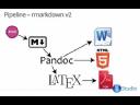
Okay, so I had mentioned that the R Markdown package has actually been around for a while. And so this was primarily the old workflow is that you had R Markdown that would render to Markdown. And then we used a tool called sundown to create HTML. And you can actually create LaTeX and PDF out of this as well. But it was kind of a more simplified pipeline.

But until we can, excuse me, show a quick example of what that looks like. So this is just an example R Markdown file I have, you can see again, most of it's just text, like I had explained before, you know, we have some special formatting, we have a couple of R chunks here. And then we're doing actually a couple more advanced features. But I won't go into the syntax of these. But just so that you can see that they are possible here, you can do LaTeX style equations, you can do footnotes, you can do all sorts of things like that. But again, primarily, the focus is just on creating prose and embedding your R code within that. So what I'm going to do is I'm going to knit that document to HTML. And you can see what that's going to produce. So this is an HTML file that happens to be shown in this RStudio viewer. But you know, we could open this up in an external browser, we could share it, send it via email, whatever we want to do. And you can see that all the conventions that we created in our Markdown document, hyperlinks, bold, any commands that we executed on the output of those commands, even any equations or footnotes with hyperlinks, you know, are all produced tables, and even graphical output from your R code.

So it's a really powerful tool, just to create HTML files. But that was primarily how the old version was used. But now, as of the latest overhaul, we actually have a variety of different formats that you can very easily get into including Microsoft Word. And so I can show a couple of examples here. Okay, so knitting to PDF, again, has been possible before, but just to show you that it works. Again, you get the equations formatted, as you'd expect, you get footnotes, you get tables, all the things that we were seeing previously, you get in PDF as well. But then, even more impressive is that all these things actually work in Microsoft Word as well. And so if you are fortunate or unfortunate enough, depending on your perspective to need to work with Microsoft Word, then you can you can easily now create documents while you're working with tools that aren't that are a little more streamlined and efficient, but ultimately produce documents that you can share with other collaborators who may want to use Microsoft Word.

So and again, as you can see, all of the conventions that we've been using actually work, there's an editable Microsoft Word equation in here that represents the equation that you produce. Again, you have your input, your output, your images, tables that you can actually go in and edit and resize and do things that you want to do with.

Alright, so many of the output formats are already defined. So we've shown you that you can do Microsoft Word, you can do HTML, you can do LaTeX or PDF. But you can also the entire system is pluggable, meaning that you can actually define a custom format and render your output into that format if you if you so desire. I'll show you the documentation for that at the end of we're not gonna actually go through that exercise just for the sake of time today. But what's interesting about this is that you can create output formats that are entirely novel. So if HTML or Word or PDF are cutting it for you, you can actually create entirely new output formats or just modify existing formats. So for instance, if you are happy with HTML, but you want your company's CSS file sheet applied to it or something of that sort, then we can certainly do that.

So I'll show you just an example, again, not of creating the the element, but perhaps if your company had certain CSS styling that you wanted, or a certain image header or something like that, perhaps you have a certain scaffolding that you want to provide around all the documents that you produce. You know, we can we can certainly do that. So just as an example, I've created a new output format. So when I go to our Markdown, or rather an output template, when I go to our Markdown from template, you can see that I've created this package, Jeff package, and it has a new template within it. So you can imagine that your company, you know, could could invest one time in producing these artifacts, and then, you know, allow other users to share them within the convenience of our Markdown. So this is the template that I defined in my, in my template. And you can see, you know, perhaps you always need to end your documents with an inclusion in this company, or if you had a certain journal that you were submitting to, and they had certain style guides for, you know, what sections you should provide, you can do that. But what's neat about this is that within my template, I've specified that there's a certain CSS style sheet that I want to be to be applied. And you can see this does not look like the original HTML document that I produced, but rather it has different colors and different fonts and things like that. So you can imagine that this could be, you know, styled for your company.

And then also you have custom formats. And so again, that's a little bit outside of the scope of what we're going to cover today. But I'll just show you a couple examples of ones that we've already produced. So if you've worked with Beamer, which is a LaTeX presentation format, that's historically been kind of difficult because you have to write the LaTeX by hand. What's great about this is that R Markdown, since it can render LaTeX, it can actually render Beamer as well, once we've defined the Beamer template, which we've already done for you. And again, this is full-fledged R Markdown. So you can do, you can embed R codes, you can embed images, you can do all the things that you're used to doing in R Markdown. And then at the end, go to knit a PDF, and you get this Beamer document that has all the content that you're expecting in it. But without having to go through the headache of learning LaTeX, or, you know, even if you know it, sometimes using it can be a bit painful. And so, you know, this allows you just to continue working with R Markdown, a very convenient and efficient and streamlined format. But you can produce very rich and complex output formats. And then also, we have different HTML slide templates. The slides that I'm using right now are actually the IO slides template that were produced in R Markdown.

All right, and then kind of the last example here, you can really go all the way with this and create, you know, entire templates that really define the entire structure of what you want to do. So you may have, you know, peeked at this when I was showing the previous template. But if you're submitting to JSS, or you're submitting to useR, or something of that sort, then you can really, you know, you can define a template that you can continue to reuse. And so if you envision yourself submitting to a journal frequently, or even if you're just submitting once, it may be worth the time to create this output template for you. So again, this is a useR submission template. And you can see that we have, you know, all the basic R Markdown stuff that we've been using up till now. But what's interesting now is that we've actually used we're using a bibliography now as well. And by providing this references section, that's going to encapsulate all of the references that we've defined here. And we're using in this case, we're just using a big tech format. But it actually supports a wide variety of different bibliography formats that you can use. So but we'll just show you this example here. So if I go to knit, I'm going to get a PDF of my useR submission. And you can see that it actually populates the bibliographies for me, it populates the citations, it does all these things that I would want it to do. And so if you're submitting to useR, this is a very easy way to do it. But but also if you're submitting to some journal that has certain conventions, you know, or certain LaTeX style sheet or something like that, this is now a much easier way to interact with them.

Interactivity with Shiny

Okay, and then the last point here, just to make this kind of a teaser, I won't go into a whole lot of detail in this, but is that now when you're using the HTML format, you can actually support interactivity. So if you're familiar with the Shiny package, that allows you to do kind of interactive web analysis within R, if I go to R Markdown, and I click Shiny, I can create a Shiny document or Shiny presentation, we'll just do a Shiny document for now. But Shiny presentations are actually kind of fun. Because you can imagine that you're using an HTML style or an HTML slideshow. But in the middle of your presentation, you have some interactive element that you can go in and kind of dig, dig into in the middle of your presentation, which is kind of a fun, fun thing to be able to do. So you can see here that this is just an R Markdown document. But if you're familiar with Shiny, you'll recognize some of these functions here of the very easy way to get into Shiny, there's really no overhead or boilerplate that's required. But when I go to run this document, I'll save it first. And when I go to run this document, you'll see that it's a regular R Markdown document, just like we've seen before, but now it also has Shiny interactive components. And so when I go through and I, you know, toggle these different, you know, widgets that I can play with, I'm able to change all these things interactively within my R Markdown document. So this is a really great way if you if you kind of envision that you're creating a largely static document, but there are little pieces where you want to add some interactivity, then this is a really nice way to be able to do that.

Okay. So finally, here are a couple of resources. And we'll make these slides and everything else available to you online afterwards. But this would be the best resource for R Markdown here is rmarkdown.rstudio.com. That will have all the details that you need about creating custom templates, custom formats, anything that you'd want to create. And then the slides are actually available here as well. The one trick here is that you'll probably want to download the latest version of RStudio. So just to for your convenience to make it easier to use all these things. Now, again, if I didn't mention this before, R Markdown is an open source freely available R package, it's downloadable from CRAN. And so you're certainly welcome to use this from any R editing environment you choose. It's just that in RStudio, we've kind of done the work to make some of these things a little more convenient in terms of, you know, just adding some buttons for you and kind of simplifying things. Great. Well, that will be all that I have in terms of R Markdown today. I'll obviously be available at the end for any questions that may pop up. But otherwise, I'll go ahead and pass control off to Yihui, who will dig a little deeper into knitr.

Introduction to knitr

All right. Hello, everyone. So today I'm going to talk about the knitr package. And you might be wondering what this title actually means. And I gave this talk at the useR conference this year. And if you are interested in that talk, you can go to this GitHub repository and find the slides over there. And for that useR talk, I assumed that you know the basics of knitr. But for this talk, I'm not going to make that assumption. So it will be a very basic introduction to the knitr package.

And so a little bit about the motivation for reproducible research. And when you do a data analysis, many of you might be doing analysis like this. So you first you write some code in your favorite programming language like R, and then you do some computing and you copy and paste results into your favorite editor like Microsoft Word or LaTeX or things like that. So you just keep on pressing Ctrl C and Ctrl V to copy and paste the results. And the problem with that approach for doing data analysis is that whenever you find a mistake in your data source, or you want to change a parameter in your report, then you will end up doing the same thing that you just did, maybe last week. So your life will be like this, you just repeat whatever you did from last week, and do all the things like clicking the buttons and copying the results and pasting that into into Word. So you certainly don't want to repeat the things. So the key solution for that problem is that you want to automate your analysis instead of manually copying and pasting the results.

So the key solution for that problem is that you want to automate your analysis instead of manually copying and pasting the results.

So to automate your data analysis tasks, you can use this idea of dynamic documents. So the basic idea is that a data analysis report is basically a combination of your program code with some narratives to explain what your code is doing here. So here is a very simple example. For example, first we write some narratives like we built a linear regression model, and then we continue writing this report with some code. So for example, here I build a linear regression model and assign that to this object fit. And then I extract the coefficients using the coif function in R. And so this will be a vector of coefficients for this linear model. And then I draw some plots for the regression diagnostics. And then I continue a paragraph and writing that the slope of this regression is this. So normally you will see a number here, for example, the slope is 3.12 or something like that, which is hard coded. But here, I don't hard code the number here. I dynamically extract the number from this coefficient vector. And when I compile this document, the code will be run, the plots will be drawn, and the numbers will be written in the final output. So this is dynamic in terms of when you want to change certain things in the code, the output will be automatically updated. So there's nothing that you want to copy and paste. So all the output will be generated automatically.

So for this talk, I will basically focus on an example for homework. So for this homework assignment, so you have some code chunks and you have some narratives explaining what your task is. In this homework example here, we were asked to find the genes that should be identified as differentially expressed, it doesn't matter if you don't understand what that means. But anyway, you read some data into your R session, for example, the data set is over here, it just consists of a bunch of numbers. So you scan that file into your R session, you set some parameters in the beginning, for example, the alpha level to be 0.05, and then you draw a bar plot. And then you do some analysis and you may also want to explain what the methods are. So for example, the Bonferroni method or the Holmes method or Benjamin and Hochberg methods. And using these methods, then you continue processing your data and draw some conclusions in the end. And we identified these genes to be differentially expressed using this method and these genes using that method. So this is a dynamic document. And when we want the output, we just click this button called knitHTML in RStudio and then the output will be automatically generated over here.

So we have a title for this report, author, dates, narratives, and some code. When you scan the data into R, you can print these values. And when you draw a bar plot using the bar plot function in base R, you will see a bar plot over here. And we have set the alpha level here to be 0.05 and that's where this red line is. So this is 0.05. And we explain these methods using some math expressions and we have a few more sections to do the analysis. And finally, we draw some conclusions. For example, we identified the gene number 1 using this method and gene number 1 using the Holmes method and genes 1, 2, and 10 using the Benjamin and Hochberg methods.

And just in case you want to change some parameters for this report, for example, I want to raise the alpha level from 0.05 to 0.2. And then if you don't use this approach of dynamic documents, then you will have to run the code again and generate a plot and paste that plot into your editor environment. But if you use this idea of dynamic documents, you just need to click a button and everything will just be updated. For example, the alpha level has been raised from 0.05 to 0.2 and the bar plot is automatically updated and your conclusions have also been updated. For example, originally here it was only the gene 1 and now we identify the genes 1, 2, and 10. So the results are changed in this document.

Chunk options and features

So just a few minutes ago there was one person in the audience who asked the question about how to hide the code. And the answer is that you can use some chunk options. For example, here I use echo equals false. That basically means I want to hide the code in the output. I only want to show the output for this code chunk. So here you only see the output. For example, here is a chunk of text output and here is the graphics output. So by using echo equals false you can hide the results. And there are some other options that you might be interested in. For example, I want to do the computing but for this code chunk I don't want to show you the results. So you can use the chunk option results equals hide and that basically means I want to run this code chunk but I don't want to show the text output. So you see when you print the p-values the printed output is actually hidden here.

So there are many, many other options that you can use. If you are in RStudio you can just hit the tab key to do some auto-completion. So there are a whole bunch of chunk options that you might want to use. And you will find the documentation for all these chunk options on the knitr website later. And that's how we can play with the text output. And actually you can also, for example, change the parameters for graphics output. For example, here the size of this plot is 5x7 inches. So if I want to make this plot taller so I can specify the chunk option figure.height equals 10 which means the height will be 10 inches. If I change the size all I need to do is just click this button again and the output will be updated.

So there are some other chunk options associated with the graphics output. For example, the device option so you can use a bunch of graphics devices like PNG device or SVG device and many others. So this is how you can play with the graphics output. And sometimes your code chunk might be time consuming so let me just show you a quick example of how you can deal with that situation. So if your code chunk is time consuming you can actually use the chunk option cache equals true. So when you turn on this chunk option the results will be cached. So you see when I click this button RStudio will pause for 5 seconds here and then show me the output. And now the second time when I click this button if I don't change the code here then it will just load the old results from the cache database directly into the R session and show you the output. So now you can see the output immediately instead of waiting for 5 seconds here.

So that's the feature for cache and let's see what else. And also if you don't want to use the R language in your code chunks you can also use some other languages using the chunk option engine. So for example here is a Python code chunk so I just need to specify the chunk option engine equals Python and then I will be able to run this code chunk using Python instead of R. So when I click this button R will launch Python to split this character string into a vector here of three elements. There are some other chunk options that can also work with the option engine equals Python and there are some other languages supported in knitr for example you can use Rcpp to write some C++ code so all you have to do is to specify engine equals Rcpp and now you just write some C++ code. Similarly just click this button and knitr will compile this C++ code chunks and show you the results in the output.

Applications and resources

So these are just some very basic features of the knitr package and you can also have some applications using the knitr package and one application is that you can build websites using knitr. For example this website Rcpp gallery is built using knitr and Rcpp so you can see this is basically like a blog site so there are a couple of posts. Seems the internet connection is not good here but you can check out by yourself later and basically this is based on R Markdown and there are some C++ code chunks in the blog posts and you can compile all these blog posts using knitr. There is also another website called rpubs.com so that basically contains a lot of HTML documents compiled from knitr. For example here is a peer assessment project one I'm not sure if that's from the Coursera course or something else but basically you can see the code chunks and the graphics and things like that. To publish to this website you can actually click this button in RStudio called publish so if you have registered on rpubs.com you can upload your reports to that website and there are a lot of other excellent examples on this website you can check out later by yourself.

Another application of knitr is that you can write your package vignettes if you are a package author so basically here is the source code for the knitr package and I have a directory called vignettes and then I have a couple of R Markdown documents under this directory. To write a package vignette using knitr you just need to specify the vignette engine to be a certain engine in the knitr package and then you specify the title for this vignette and when you compile this package and install it you will see a list of vignettes like this. So here are the built-in vignettes in the knitr package. So I just want to show you one of them which is this one called the Dockel classic style. This is a very interesting layout in my eyes. So for this layout you can see the narratives and the code and the output are arranged side by side. So if you want to hide the code you can just press the key T on your keyboard so you can just read the narratives and graphics output and if you want to hide the narratives you don't care about narratives you just want to read the code you can hide the narratives and just read the code. And for most people probably this side by side layout is most appropriate. So this is how you can play with the Dockel style in knitr.

So there are a couple of resources to learn more about knitr. The first one I want to recommend is just the online documentation for this package which is at ua.name.knitter. And if you are just too rich you can just buy this book I wrote last year Dynamic Documents with R and knitr but you don't really have to buy that one because I have very comprehensive documentation for this package online.

So just a last comment on reproducible research which is the topic for today. So reproducible research is really not a trivial thing. I mean there are a lot of things to consider when you write a report. Just by using knitr does not guarantee that your report is reproducible. For example you might be using some absolute paths in your reports which will not be reproducible on other people's computers. There are just a lot of things to consider. But I guess knitr will be helpful at least as the first step to reproducible research. So I just hope all of you can be patient enough to wait for this area of reproducible research to grow just like this tree. And finally hopefully we will be living in a wonderful world of reproducible research. Thank you.

PackRat: dependency management for R

Thanks Yihui. So now I'm going to talk about PackRat which is a dependency management system for R. So given everything that Jeff and Yihui have taught us about trying to write reproducible research. One thing that we want to be able to do is take the R environment that we use to produce these reports and try and preserve that over time. So PackRat is an R package that helps us manage these R projects, R package dependencies in a way that is reproducible.

So when you form an analysis you're going to use different R packages. Say you got them from CRAN or if you live on the bleeding edge maybe you got them from GitHub. But when you do an analysis or write an R project you want to make sure that you can save these packages over time. Say you publish this as research and one or two years down the line you need to run that again. You want to make sure you can reproduce that exact same results with the exact same environment that you used originally when forming the analysis. Another thing about this is you want your projects to be isolated. So in the current state of the R world when you install a package it goes into your global library. So every project that you write on your computer has access to that package and that's often useful. In some occasions you want to be able to have a private library for each project in case one project depends on one version of a package and another project depends on another version of a package. So PackRat gives you a means of isolating these package dependencies within a library for each project. And last of all we want this to be portable so that if you need to collaborate with people on alternative machines they can build the same R environment using the same system from your PackRat project. So PackRat makes it easy to install those packages for a particular R project.

Part of the reason why the PackRat development was motivated is for those of you who have either been in research for a while or done some work and come back to it a year later. You've probably come back to your code and asked first of all who wrote this garbage code? Unfortunately one of the side effects of becoming a better programmer is realizing that the code you wrote before is probably not as good. And unfortunately if you come back to code a year later unless you wrote it in a reproducible nicely commented way you're going to struggle to recollect exactly what you did and how you did it.

Another thing is you might have used say Lattice which is an R package for generating plots. You used that to make some figures before. But now when you try to run it with your new version of R, say you updated it recently, all of a sudden your plotting code is just throwing errors at you. For some reason a Lattice update has broken your code and you know your code didn't change but Lattice did. So now you have to figure out what changed and how you can fix your code or find the old version of Lattice. Say you used the NLME package for fitting non-linear mixed effects models. And when you ran it before everything went fine. You showed the results to your boss or you published it as research. The model convergence criteria everything worked okay. You come back and try to re-run it a year later and something has changed underneath NLME and suddenly it's complaining about model convergence. I guess something changed in there and how they are fitting the parameters and this makes you feel pretty uncomfortable. Suddenly the environment you used to produce the results before, you can't reproduce that with this new environment with the updated version of NLME.

Another one is not every R package you use is going to be on CRAN or GitHub or an external repository. Say you got it from collaborators who put it and they just share it through email or you got on a USB stick from someone. You really don't want to have to go and hunt that back down. It'd be really nice if we were able to just keep that package in a project and save it over time. So PackRat helps us solve this problem by one, we make sure that package sources are stored alongside your project. And we track the package version so that if you update R but you need to return to an old version of a R project, you can roll back and reinstall that package for some reason. So the way I like to think about it is PackRat lets you build the sandbox in which an analysis can run and it helps you ensure that this sandbox will persist over time.

So the way I like to think about it is PackRat lets you build the sandbox in which an analysis can run and it helps you ensure that this sandbox will persist over time.

And as I said before, one of the benefits but also problems with the current system for R packages is that everything gets installed into a global library. So all projects on your system have access to the same library. But for a particular version of R, only one version of a particular package can be installed at a time. This is problematic if you have multiple projects on your system and one depends on a current version of a package, say R3P. And another one depends on a newer version of R3P which maybe doesn't work with your older one. But you want to leverage the features of that for new projects. So we want to be able to isolate these package dependencies for each project and PackRat helps us do that. So PackRat does this by giving each project its own private PackRat library. So if you don't know what a library is in R parlance, a library is just a folder of installed R packages. So when you make a call to the library function which is kind of poorly named because it loads a package from a library. Say we use library dplyr to load the dplyr package from the library. R will attempt to load dplyr by default from that global library. If you use PackRat to manage an R project on the other hand, PackRat will ensure that R loads that package from a private library instead.

The other nice thing is because we do it this way with PackRat, it doesn't interfere with any normal workflows. Any calls to install.packages, devtools install github, bioclite if you're a bioconductor person. These will also get installed into the private library. So you can ensure that installing new packages for one project does not break any analysis you have for another project. And because PackRat collects all of these project dependencies and it ensures that it is portable across different systems. So if you're working with collaborators, you can ensure everyone working on a project is using the same version of any R packages your project depends on. So you don't have to worry about, oh you're getting a bug, is it because you have the newest version and I'm using this different version of this package. When people collaborate on a PackRat project, you ensure everyone works in the same environment.

PackRat demo

All these things are better done with a demo, so I'll switch to RStudio. So let's start a new project in RStudio. So with the latest RStudio daily builds, we have really nice PackRat integration. So the first thing you'll see is, let me go back. If I go to start a new project from a new directory, an empty project, we now have this new tab, Use PackRat with this project. So let's say I'll make a new project called Omelettes because I want to analyze different ways of making omelettes. So I do this, PackRat does some work to set up the project here, and RStudio bumps us and we have a new project. So we're in the Omelettes project and everything looks the same as before. The only thing that is slightly different now is if we go over to the packages pane, we'll see that we now have two libraries, two places where our packages live. We have the PackRat library and we have the system library. So what we have done is we've isolated any dependencies and everything we install is now going to live in this PackRat library.

Let's say I want to use StringR for some bit of code that I'm running here. So first of all, I don't have StringR. It might have been in my user library, but because I'm using PackRat, that library is hidden from us. So we're going to go and make sure that we install it. And notice that it gets put right into our PackRat library. So we have StringR from CRAN version 0.6.2. And you might have seen that PackRat immediately took that and said, oh, I see you installed a package StringR. I'm going to track that. I'm going to track its source. And so you have this package in your library and you have StringR in your PackRat private library. So now we can use StringR.

So let's say we don't want to wait for that. So you see, as the packages are installed, you're getting PackRat to track them. So now these packages are tracked in our PackRat library. And sorry, I'll go and get dplyr once more. The initial bump of getting the packages in your PackRat library is a little bit slow, but it's worth having your project reproducible over time.

Kevin, we're getting a few questions about the size of the PackRat repositories. Can you comment on how big you'd expect these to get? So with PackRat repositories, yes, they will grow in size because you keep all of your package sources and you keep a library of packages for each PackRat project. So they do get a little bit bigger, but by default, if you want to rebuild or share a PackRat project, all you need is the PackRat lock file. You'll see there's this PackRat.lock file, which tells you what version of a package you have and what its source was. If you trade that around, that's all people need to share and restore a package.

So now, suppose I call PackRat status. It tells me that everything is up to date. Now suppose I remove a package that my project depends on. Say I remove dplyr now. So notice how in this file here, I'm calling dplyr. So I have my project needs dplyr to run. And RStudio will go and say, hey, you're using dplyr on your project. I saw it was removed, but you're using it. So I think you probably want it in your library. So it instructs you to update the library. It tells you that these packages have changed in PackRat and you can use restore to apply these changes, which restores the library based on the state of your PackRat lock file or the last snapshot. So we do that. We see that a call is made to PackRat restore. So restore takes the last consistent state of your project and applies it to the library. So it's reinstalling dplyr from CRAN and unfortunately, I'm compiling from source, so it's a bit slow. Normally, if you're running a CRAN build of R, this won't be a problem. But the point is here that PackRat tracked dplyr. It knew what version it was. It knew where to get it. And so it can go out, grab the package and install it or install it from local sources as all the PackRat package sources get cached as well.

So we also see that, you know, if we didn't have access to the Internet in dplyr, we have the exact package sources for dplyr version 0.2 to use as well. One of the things that we saw earlier was we have this idea of what is known by PackRat, which is shown in this column here. And what is currently in your library, which is right here. And normally, you have the action PackRat snapshot for taking the state of your library and applying it into the PackRat lock files. You say, I want to preserve the current state of my library over time. And PackRat restore for taking the state of the last consistent library state and applying it to your library. But right now, because we're a consistent state, both of those actions do nothing.

One thing, the two things you need to know about to use PackRat is the snapshot, the current state, the current consistent state of your projects are dependencies and the private library of packages that power your project. So we have two main verbs for interacting with these two components. PackRat snapshot records the package versions used by a project and downloads their source code for storage with the project. And PackRat restore applies the previous snapshot to a project, building packages from source as necessary. So once you have your project in a consistent state, you want to save the current state of the world, use PackRat status to do that. If you want to restore that previous state, say you've removed packages or you received something from a collaborator, use restore to restore the library.

So I went through that demo. So we saw these init to initialize a PackRat project. PackRat saves the current state of your library to the lock file. Restore restores the lock file to the library. We saw this on the RStudio new package call. We call snapshot. It takes the current state of the library and saves it to the lock file. We call restore. If we've lost those packages, it restores them based on the state of the lock file. Now, I didn't show it in the demo, but we can, of course, use packages from GitHub. So we have a PackRat function or DevTools function for installing packages from GitHub. Say we want to use the development version of RCPP. We can do that and we would get the development version, which if we had a previous version from CRAN, we'd see that PackRat is upgrading it from the CRAN 0.11.2 to the development 0.11.2.1.

The last thing we can do that makes it easy to share projects is we have bundle and unbundle. So bundle packages up every file within a project along with the parts of the PackRat ecosystem that are necessary to rebuild the project. And you have control over whether you want to include the package sources or the package library, which you usually don't want to do. You want to rebuild that on other systems if necessary. But you can include the sources if you want to have them locally for rebuild. The other thing is we expect PackRat to work nicely with version control. So the PackRat lock file keeps the last consistent library state. But if you're tracking a project with GitHub, you can track that lock file over time. And so you can roll back to any state from a lock file within that project if you need to. The main goals or objectives of PackRat is to create a nice little environment for your R projects to run and live in and keep that reproducible over time. And we want to make it as easy as possible to use both from PackRat and from RStudio to manage your R dependencies over time. And of course, right now we only manage R package dependencies, but there are also other software for managing entire operating systems or environments. For example, Docker, if you're interested in that.

And so currently PackRat is not yet on CRAN. It is only available on GitHub. So if you want to install the latest version of PackRat, you can close this project. And if you have the DevTools package, you can install it with a call to DevTools install GitHub. And so that'll go out and grab it and install it. So now you have it available for use with any projects on your machine. With that, thank you very much for joining us on the reproducibility webinar. And we'll be here to answer any last questions that you have about Jeff, Yihui, or my presentation.

Q&A

We had a number of questions. JJ and others have been very active answering them. Maybe there are a couple that are worth trying to answer very quickly because there were sort of themes. So one of them, Kevin, was how does this support... What about if you're using different versions of R? So PackRat does record the version of R in a library. So unfortunately, PackRat doesn't do the grunt work of finding the version of R for you, but we do record it. And so if someone is using a different version of R and they try to open your PackRat project, PackRat will warn them. And unfortunately, we don't find R and install it for them, but they know that, oh, this project was using this version of R. I should probably go and find it just so I ensure that the environment matches that the project was built in.

Great. Thanks. Hey, and going back to you, Jeff, at the very beginning, a number of questions. You know, anytime you're talking about outputs, the program that controls those outputs has a lot of functionality like Word or even PDFs. And so there were some questions. I'll raise one in particular. What about interactivity in PDF documents? Yeah, interactivity doesn't work within PDF documents because the interactivity is really, that's a web application that's running inside the browser. And the PDF document isn't able to host a web application.

Yes, and there were similar, you know, some questions about, you know, Word and tracking changes. And, you know, there are details here that matter, and you'll want to read the documentation. It's not, you know. Yeah, the website, rmarkdown.rstudio.com, has a ton of details about all the formats and what, you know, what features are supported, what works, what doesn't work, all that sort of thing. And as we hit the hour here, last question I would call out. The differences between, because not only did I see it on this session, but I also saw, I've heard about it from others. But sort of, you want to cover, or somebody want to cover the difference between knitr and RMD and rmarkdown?

Okay, so I didn't actually mention the other document formats that knitr supports. Actually, in the very beginning, knitr started with the document format called RNW, which basically means the combination of R and LaTeX. But as time goes on, people seem to be interested in rmarkdown, much more interested in rmarkdown instead. So, actually, if you are comfortable with LaTeX or raw HTML, you are free to write these kinds of documents. Yeah, for the rmarkdown document, for the rmarkdown package, it's basically a wrapper for the knitr package and the pandoc converter. Okay, thanks.

And we're out of time. I'll just throw it out to you guys. Was there anything you wanted to, you know, any issue that came up in the Q&As that you wanted to call out here that we have an opportunity to say it to the group? All right, folks, we thank you very much for attending today. We'd love for you to check out all of our products on our website. You can see here some links to our evaluation products for our commercial ShinyServer Pro and RStudio Server Pro products. We'd certainly appreciate you looking at those. And with that, we'll call it a webinar and look forward to seeing you on September 3rd.