Data Wrangling R | RStudio Webinar - 2016

So I've prepared some slides sort of off the cuff for the webinar today, and it's all about data wrangling. And one thing I'll point out after I introduce myself, I'm Garrett Grollemund, and I work for RStudio, and I write books on R and teach people how to program with R. And all the slides I'm going to show you today are available online. They're available right now, so you can download them or later. They're at this link at the bottom of the slide. But I put that link in the slide template, so it'll show up on any slide. If you want to follow me on Twitter, there's my Twitter address, and also my email address if you have any questions you'd like to follow up with.

This webinar will go through two packages that Hadley Wickham, my colleague, made, and they're both really geared towards working with the structure of data. So that's the tidyr package and the dplyr package. And then what I'm going to cover today really follows closely a cheat sheet that we published a couple days ago. So this is a cheat sheet you could download at the link at the bottom of the slide here, and it's a two-page sheet that just summarizes the tidyr package and the dplyr package. So it's a great resource for remembering the functions that we're going to go through today, and also for just remembering functions in general as you work with data.

Ground rules: tibbles and the pipe operator

So before we really get into data wrangling, there's a couple of ground rules that I want to familiarize you with. So these two packages introduce some things into R that makes R work better, but also makes R look a little different. So I just want to make sure you're comfortable with that before we start using them. And the first is the table structure or table TBL. And what a table is, I'm going to say table because I don't like table, but it's just a data frame basically, you can think of it as a data frame, that appears differently in your console window.

So for example, if I go over here to my R window, this is just a RStudio window that I put off on the side here, and I open up a familiar library like ggplot2, there's a data set in here called diamonds, which is humongous. And if you try to look at this data frame, well this is what happened, it fills up my screen and at some point R tells me that it's not going to show the rest of the data. This data set is 52,000 rows, and really what I do see here isn't very helpful. A, it fills up my memory buffer, which means I can't see what I did before, and B, I can't even see the names of this data frame. So what a table is, is a new class that you could give to a data structure like diamonds.

And it's implemented through the dplyr package. So I can change diamonds into a table with this function table underscore dia. And now I have the same data frame here, but the print method is only going to show me the part of the data frame that fits in my console window. So it's showing me right now that there's a variable called y and a variable called z in the diamonds data frame that went off the side of the window. Instead of wrapping them below, R now is just going to tell me these variables are here but they're not shown. And then instead of showing me 52,000 rows, it's just going to show me 10 rows. So this is a more pretty way to look at your data.

So there's a function I recommend to use when you want to look at the entire data set, and that's the view function. It's in Base R, and if you call it from RStudio, RStudio will open up a spreadsheet-like view window where you can check out your data set, almost as if it were an Excel document. Keep in mind that's view with a capital V, and you can use this on any data frame that you have in R.

Then there's one last function that really changes how R looks, and that's the pipe operator. This comes from the Magruder package, but it's imported by the dplyr package, and it's a different way to write the same code that you'd write before. So you can probably recognize what this command would do here. We haven't looked at select. We'll look at that today, but it's calling select on an object called tb, and then it has some arguments here. The pipe operator allows you to pipe in the first argument of select, so I'd write tb pipe select child to elderly, and what the operator will do is it'll insert tb as the first argument of select, so these two lines of code would do the same thing.

So at this point, it might not be obvious why you'd use pipe over anything else, but the cool thing about this format is you could start chaining arguments together. As your chains get longer and longer, this becomes much more efficient than actually managing where you save the in-between states.

What is data wrangling?

So let's take a look at the functions that can actually help you wrangle data, and what I mean by data wrangling is what other people call munging or transforming your data or manipulating it, and the reason I use the word wrangling is it sort of captures how painful this process can be. So there's an article we link to in the registration email from the New York Times that said that about, you know, 50 to 80 percent of the data scientist's time is spent doing things like munging and wrangling their data. It also offered a new word for data wrangling, which was data janitor work, which I found amusing. So I don't know where they got this statistic from, but I think a lot of people would say that just getting the format of your data into a format that you can work with is time-consuming, and it's often boring and painful, and if you could do that more efficiently, that would be a big win, and the functions we'll look at today will help you do that.

just getting the format of your data into a format that you can work with is time-consuming, and it's often boring and painful, and if you could do that more efficiently, that would be a big win, and the functions we'll look at today will help you do that.

Normally when you wrangle your data, you have two goals. First, you might need to make your data set suitable to a particular piece of software. For example, we're going to need to make our data suitable to R because that's what we're using, and then second, you can actually reveal information by changing the format and the structure of your data.

Tidy data

Let's start with this first goal, making our data suitable for R. So your data sets can come in many different formats, but there's one that R definitely prefers more than the others, and I have some toy data sets in this package, which I built on GitHub. You can download it if you want to use these data sets. It's completely not necessary. I'll be using these, and you could just sit back and watch, but should you want to install this package, first install the devtools package, which is on CRAN, and then use the install github command in devtools to install this from the link rstudio-edawr.

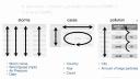
Inside this data frame, inside this package, I have some data frames that are all fairly small, but demonstrate the sort of layout and formatting issues that you might encounter with data in R. For example, here are three data frames from the package. One's some data about hurricanes in the Atlantic Ocean, one's some cases of a disease, in this case TB in different countries in different years, and one's some data about pollution. And we could go through these three data frames and try to analyze what they contain. In particular, we could look at what variables are in each of the data frames. In the storms data frame, it's pretty straightforward. We have a variable that talks about the names of each of our storms, a variable that has something to do with the wind. It's actually the maximum wind speed recorded for each storm, a variable that records the pressure of each storm, and the date on which these measurements were made.

If we turn our attention to the cases data frame, we'll see that we have a variable that has some sort of country code, so we can see France, Deutschland, and the United States there. We have a variable that lists different years, 2011, 2012, 2013, and we have a variable that's left over that's something like a frequency or a count, or you might just call it n. And if you compare cases to storms, you can see already that we have the difference between the two data frames. They store the values of their variables in different ways. In storms, each variable is put in its own column. In cases, one variable is in a field of cells, one's across the column headers, and one's in its own column.

When we get to pollution, we see a different format still. We have a variable that's different city names, and then it looks like we have a variable that describes particle size and a variable that describes some sort of amount, but I think you can also argue, and this is what I would argue, that we actually have a variable which is the amount of large particles that each of these cities has in its air, and the second variable which is the amount of small particles that each city has in its air. And if you wanted to compute some number for each city, like the ratio of large to small particles, then you'd have to treat these things as separate variables to do math with them.

But if you looked at how you'd pull the values of these different variables out of these data frames, you'll see that one of these formats is much nicer with R code than others. In the storms data frame, you could pull out each variable using the same syntax, the name of the data frame, the dollar sign, the name of the column that you want. But if you want to pull out the values of, say, the count variable from cases, you'd actually have to extract a bunch of cells and paste them together in some way. And this is bad because when you write your code, you want to be able to make it as generalizable and as automated as possible. And if you have to stop and look at the data set that you're working with, and then think about how to extract the values of the variable you want within that data set, well then it's going to be really hard to write a piece of code that will work with other data sets as well. So just due to the way R works, its syntax structure and everything, it's much easier to work with your data if each variable is in its own column.

But there's other advantages as well. If we look at the storms data frame, and consider making some sort of new variable, in this case, the ratio of pressure to wind. Meteorologically, I don't think that's a meaningful variable, but this is similar to things you do with your own data. You'd use some math like this in R, and what that code would do is it first extract the pressure variable storms, and then it would extract the wind variable, and then divide the two. And the way R operates is it's going to do element-wise operations. So instead of doing some sort of linear algebra thing here, it's just going to pair up the first value of each vector, the second value, third value, and so on. And so we get a vector that has, at the end, just as many values as the original vectors.

Now this is great if you put your data in such a way that each variable is in its own column, and then each row contains a single observation. Because what element-wise operations will do is it'll make sure that the values of one observation are only paired with other values from the same observation, which as a data scientist is just what you want. We wouldn't want to divide the pressure of Alberto by the wind speed of Alex. That's really not a meaning for the quantity. So we want to make sure we keep the pressure of Alberto with the wind of Alberto, and the pressure of Alex with the wind of Alex, and so on. Well, the structure of the storms data frame makes that happen automatically.

And I'm going to call that data structure tidy data. This is a term invented by or popularized by Hadley, the author of Tidy R and Dplyr. And what it amounts to is you take your data, and you make sure that each variable is saved in its own column, which we saw storms did. You make sure each observation is saved in its own row. And then finally, you want to put basically all the data that you plan to work with in the same data table before you start working with it. Otherwise, you'll be recombining your data every time you make some sort of adjustment to it.

So, if you make your data tidy, with variables and columns, observations and rows, and the type of data in its own table, it will be easy to access your variables, and you'll automatically preserve observations as you do things to your data. So, that's sort of the goal. Tidy R is the means to get there.

The tidyr package: gather and spread

The package that picks up where reshape2 left off, if you are a user of reshape or reshape2, and tidy R has two main functions, gather and spread, that do similar things as cast and melt, if you're coming from the reshape world. And then there's several other functions we'll look at in there. But these are the main ones, and let's take a peek at them.

So, this is the cases data frame. This is how the variables were distributed. What I'd like you to do, and just for 30 seconds, because I can't really check in with you guys or communicate with you, imagine how this data frame would look like if you restructured your data. If you restructured it to be similar to storms. If it was tidy and had the variables country, year, and end. I think if you tried to scribble this out on a sheet of paper or something, it would make it much easier to follow what gather does, which we'll look at in a second.

All right. So, hopefully you had a chance to imagine what this data would look like in a different format. And this is what I propose this data set would look like in a tidy format. We want to keep all of the information in the data set, and we want to keep the variables that are there and the values that are there. We just want to restructure them so the variables each appear in their own column. And we know that the columns we want to end up with are something like country, year, and end. And we can also look at the old data set to determine what values need to go in which rows of the new data set. We need to have some combination of France, the year 2011, and the end value for that combination needs to be 7,000. And basically, we need to port over all the values in this field of cells into our new data frame. And when we're done, our data frame will look like this. So, this is a tidy version of the case's data frame. Now it's very easy to pull out each of these variables by selecting the column name. And we can do this sort of thing with the gather function.

And before we do, we want to develop one piece of vocabulary. So, if you look at the output, we see it basically took the right-hand side of this data frame and turned it into two columns. The first column is a key column. These are the names that these cells had in the previous data frame, the column names. And we'll call the second column a value column. So, these are actual values that appeared in that field of cells. And the idea of a key value pair is actually pretty common. So, we're going to use gather to take a cells and turn it into just two columns, a key column and a value column.

This function comes with the tidy library. And you first get the name of the data frame that you want to clean up. And then you give it the name that you want to use for the key column that results in the name that you'll use for the value column. So, we happen to be moving column names that were years into its own key column and cell values that were, you know, N for frequency into their own column. But, you know, gather and tidy R can't know what those things actually stand for. So, here we get to tell them what to name the new columns. Then finally, we just tell gather which of the columns we want it to use when it builds those final two columns. You may remember in the cases data frame, the first column was already tidy. The countries were already in their own column. So, we don't include one in this index here. We leave one be. We just include two through four. Those were the columns that were not tidy. When you do this, your data will go from here to there.

So, this is our pollutions data set and it has three variables distributed like this. We can make this data set tidy with a column called city, a column called large, and a column called small. Before we do, try to picture in your mind what that would look like, which will help you understand the goal we're working towards in the next few slides.

All right. So, the cases data frame looked like rectangular data. That's the sort of data that you'll find very often when you only have a few variables and you want to display them in a format that fits in a paper pretty well. I don't know what to call this sort of data, but it exists quite often as well. And if you can switch this sort of data and rectangular data, you pretty much have full control over the format of your data frame. So, here's the pollution data set as it is. We want to make it a data frame that has these columns in it. And just like before, it's only a matter of recreating the combinations that appear in the original data frame in our new data frame. And when we do that, this is what the result looks like. See, it's tidy. It's more rectangular than the previous data frame. Now, there's fewer rows. We've removed some redundancy here.

When we did this operation, we again were working, you could think of it as working with a key column and a value column. The operation that we're going, the function that does this operation is called spread. And what it does is it looks at the original data set, and you give it a column to use as a key column, and a column to use as a value column. And it'll use those columns to recreate a field of cells. But the way you call spread is, the idea would be that the field of cells you recreate will be a tidy field of cells. The syntax for spread is, you give it the data frame you want to reshape. You give it the name of the column used as a key column in the original data, and the name of the column used as the value column in the original data. Here, that's size and amount.

You could think of spread as taking data that's in a key value column format and putting into a field of cells format or rectangular table format, whatever vocabulary you like. You could think of gather as doing the opposite. And by going back and forth between gather and spread, you could actually move values into column names, out of column names, variables into a rectangular format, a tidy format. And since you don't have to apply spread or apply gather to the same columns each time, just by iterating between these two functions, you can take the same data, preserve all the combinations in the data, and make the layout very, very different than it was to begin with.

Separate and unite

So the tidier package also has two other functions that I think are useful, but not always going to be that useful. If you looked at the storms data set, and you're very persnickety, you might notice it actually has three more variables in there. You could extract a year variable from the date, a month variable, and a day variable. And those variables are all combined into one column here, the date column. What separate does is it takes a single column, and it splits it up into multiple columns based on some sort of separating character. So this is really easy with dates, because dates normally have some sort of separator between year, month, and day. And if we ran this code above here, we get a new data frame where the date column has been split into a year, month, and day, three columns. If I save that as storms2, then I could use unite, which does the inverse. It takes several columns and puts them together in the same column, adding a separator between the values of the previous columns. So that's a great way to recreate some dates. Although in this case, those dates would be character strings, you need to reparse them if you want them to behave as dates in R.

So just to recap about the tidy R package, it primarily works with the layout of your data, reshapes the layout. Use the gather function and the spread function to change the shapes back and forth. They're complementary. And then you can use separate and unite to split up and unite columns. They're also complementary. This package is designed basically to get data into that tidy format, which is the most efficient way to work with it in R. But let's turn our attention now to the dplyr package, which has a different design.

The dplyr package: select, filter, mutate, summarize

Datasets contain more information than they display, and dplyr is designed to help you sort of access that information.

So you'll need to run library dplyr before you can use the functions in this package. You'll also need to install the package, of course, if you want to use it. The main functions that we'll use for manipulating data are listed here in their help pages, but we'll just go through them one at a time. So when it comes to accessing information in your data frame, it can help to just extract information that's already there to avoid the sort of overwhelming amount of distraction that the other variables provide. So you can extract variables, you can extract observations, you can derive new variables, and you can change the unit of analysis that the dataset displays. dplyr provides four functions, each dedicated to doing one of these things. And let's take a look at them, starting with select.

So select is very simple. It's a way for you to just pull out variables or columns from a data frame. So if I only wanted the storm column and the pressure column from the storm's data frame, then I could select from storms, the storm and pressure column. And you could list as many column names or as few column names as you want there, and it'll bring back everything you list. So that's easy enough to do in R. You might ask, why would you use select to do it? Well, one thing that select does is it provides more ways to specify which columns you want. So you'll know that if you use brackets and integer subsetting, you can put a negative sign in front of an integer, and that stands in R. With select, you can put a negative sign in front of a name, and you'll get back everything except that name. You could also use the colon notation to get a range of variables. So this would say, giving back the win variable, the date variable, and any variable that appears in between them.

Filter is analogous to select, except instead of selecting columns, it brings back rows, or if your data is tidy, these would be observations. And the way filter works is you give it a logical test. So here I'm giving it the test where wind is greater than or equal to 50. What filter will do is it'll apply that test to each row in your data frame and give you back just the rows that pass the test. You can combine tests by putting a comma in between tests, and what filter will do is it'll combine them as if there is an and statement between them. So these are only the rows where the wind is greater than 50, and the name, the storm name, is in Alberto, Alex, and Alice. If you want to do an or condition, we'll just use the boolean operator for or and r to combine two tests into a single test.

The mutate function takes your data frame, and it returns a copy of the data frame with new variables added to it. Normally, these will be variables that you derive from the variables that exist in your data. So before, we had sort of the bogus example of calculating a ratio variable from the wind and pressure variable in storms. The information in that ratio variable was in the data to begin with. It just wasn't on display, but you could logically derive it from the data frame. You run mutate on the data frame you want to add to or change, and then you give it the name of the new column you want to make, and you set that equal to some expression that will make the values of the new column. You can make more than one column at the same time, and you could even use a column to make a new column in the same command. Make sure that the first column appears before the columns that rely on it.

This command, mutate, doesn't actually affect your original data frame. It returns a data frame that has the new variables added to it. So if you want to save that data frame and use those variables later, you'll need to assign it to an object. There are a lot of functions that are useful to use with mutate to make new variables. This is a short list of them. And each of these functions has something in common. They all take a vector and return a vector the same length. So if you want to add a column onto your data frame, that column's going to have to have values for each row in the data frame. You can call these window functions, because they sort of pass the whole vector through a window, and the vector changes, but each element is still represented at the end.

Okay, so the last of those four functions we listed was summarize. And summarize takes a data frame and it calculates summary statistics from it. You get back a new data frame, and usually that new data frame is much, much smaller. For example, here I'm summarizing the pollution data frame by calculating the median value of amount. I only need one value to show the median, so my new data frame only has one row. Summarize works similar to mutate. You give it the name of the new columns you want in your new summary data frame, and then you set those names equal to the R code that will build those values. Like mutate, there's functions that seem to work best with summarize, and things like the standard statistical estimators, min, mean, variance, standard deviation, median. And all these functions are similar to each other in an important way. Unlike the window functions used with mutate, these functions actually all take a vector or a group of numbers and return a single number. So you could think of them as summarizing functions or summary functions.

Arrange and the pipe operator in practice

There's one more function in dplyr that doesn't really add to your data or subtract from it, but you can consider it like a fifth horseman of dplyr, and that's a range. What a range will do is it'll rearrange the order of the rows in your data frame based on the value of one of the columns. So here I rearranged the rows in storms based on the value of wind. And if we color-coded this data set, you could see that it's easier to see that whereas before the rows were not ordered by wind value, now they go from the row with the smallest wind value to the row with the highest wind value. If you wanted to reorder them in a different way, in descending order, you could use this helper function DESC, it stands for descend, and just wrap that around the variable whose values you want to be ordered from highest to lowest. If you give a range one variable, it'll arrange based on that variable, and ties will just occur in the order they appear in the data frame. But if you give it a second or third variable, a range will use that variable as a tiebreaker variable within rows that have the same values of preceding variables.

Okay, so I mentioned that pipe operator earlier, and this is where it really starts to come into play. And then if you use the piping syntax, it's very simple to pipe the results after one expression into a second expression. So if you wanted to first filter the rows to extract all the rows for wind speed 50, and then take those results and select two variables from it, you could just add a second pipe operator in the select command at the end of your code. If you then wanted to mutate that data frame or summarize it, well then you just add a third pipe operator in the next line, and so on, and so on. So it becomes very easy to build up this sort of record of what you're doing to transform your data, and it's very easy to add to that record. And then if you read through what we're doing here, I think this way of reading code is actually very transparent. Take storms, then filter it to just the rows for wind speed 50, then select from it storm and pressure. Just read the piping operator as thin, and I think it makes your code very legible.

Group-wise operations with group_by and summarize

This is our pollution data set. It describes pollution particle amounts in three different cities, and we could calculate the mean amount, the sum of the amounts, and the number of rows in the state of frame, and put them in the summary data set. If we look at that summary data set on the side there, well, all right, let's look at pollution first. You'll notice it's a tidy data set. It has variables, it has observations, and if you look at the summary data set, it also has variables, in this case three variables, and it does have an observation, just one observation. But each of these things, the mean, the sum, and the end, each of those values describes the same thing, and that should raise the question, what is it that those values describe? And if you think of a mean of 42, or a sum of 252, or even an end of six rows, it becomes pretty clear that what they're describing is this entire data set. It's almost like we've made measurements on data set, we've made an observation on the data set, and all data set is is a grouping of observations, or grouping of rows.

So if we make observations on an entire data set, well, then we could also make observations on subsets of a data set. We can make an observation on six rows, why not make an observation on two rows, or three observations on two rows? And if we did that, then we could have means, sums, and ends that are keyed into, in this case, different cities, you know, the mean amount for New York, the mean amount for London, the mean amount for Beijing. You can do this sort of thing, this group-wise operation, by combining the group-by function, which comes from dplyr, with the summarize function that comes from dplyr.

Here's how it works. If you run group-by on a data frame, and then you give group-by the name of a column or variable, it will add some metadata to the data frame that tells R, or tells dplyr, what the different groups of rows are in the data frame. In this case, it will group the data into three groups, one group for each unique value of the city variable. Now, at this point, it doesn't do anything. If you just ran this, that metadata will stick around with your data frame, and dplyr might use it if you run a dplyr command on that group data frame. The magic happens when you combine a group data frame with summarize, or mutate, or filter, or whatnot. What dplyr will do is apply summarize in a group-by fashion, or mutate in a group-by fashion, and so on, where it makes sense. So here, if I first group by city, and then summarize to calculate a mean, sum, and end variable, dplyr is going to split the data into groups, conceptually. It's going to apply the summary to each of the groups separately, and put those summaries back together into a final data frame, and this will be my result. This is how you can get group statistics, or group-wise summaries from your data.

The magic happens when you combine a group data frame with summarize, or mutate, or filter, or whatnot. What dplyr will do is apply summarize in a group-by fashion, or mutate in a group-by fashion, and so on, where it makes sense.

You'll notice that the three variables I calculated with summarize, mean, sum, and end, are in the final data set, but to those, dplyr has added the city variable, and that variable came from the grouping criteria, and it's necessary for dplyr to add each variable that's involved in the grouping process, so we know what the values of mean, sum, and end refer to.

So if we put this process together, this is what it looks like. We take our data, we group it, and we get group-wise summaries. In this case, I'm only taking the mean. Here, I'm grouping by size. Before, I was grouping by city. The rows don't have to be near each other in a group. Everything will just be grouped together based on common values, wherever those values appear in the data set. Once you have grouped data, you can remove the grouping information with ungroup.

So this data set doesn't actually exist. There is a TB data set in the EDAWR package, but it's much more complicated than this one. This is a simplified version. But you can imagine, we could take this data set that has different countries, different years, different genders, number of cases of TB. Anyways, we could group it. In this case, we could add more than one variable to the grouping criteria, and what groupby will do is it'll create a separate group for each combination of those variables. So for example, Afghanistan in 1999 will be one group, and Afghanistan in 2000 will be a separate group, and so on. And then we can run summarize on that. And what we'll get is our summary. But when you run summarize on grouped data, summarize will strip off one variable from the grouping criteria. So now that it's made the summary, it's going to strip off the rightmost variable. In this case, that's year. And what you'll end up with is a data set still grouped, but it's only grouped by country. It's no longer grouped by country and year.

By stripping off just the last grouping criteria, this will be grouped by country, and we can immediately run summarize on it again, and this time get summary statistics based on the different countries. And now let's go peel off that variable country, and the data is no longer grouped after we've summarized a few times. So this process of grouping by many variables and then summarizing, peeling off one level of grouping criteria as you go, is a way to change the unit of analysis that your data looks at. For example, we can use the process to make these four data sets here. They all come from the original TB data, but one of them is really describing combinations of, in this case on the left, country by year by sex, and then we change that to just country by year, and then we change that to just country, and then we change that to the entire data set. And different types of information can become apparent at different levels of grouping here and summarization.

Combining data sets

So I know it's been a lot. This is definitely going to be a whirlwind tour, but we're near the end. You can extract variables and observations with Select and Filter. You can rearrange your data with Arrange. You can make new variables with Mutate, and you can make new observations on new units of analysis by combining Group By with Summarize. So there's one last thing that you will probably want to do as you wrangle your data with these packages, and that's combine multiple data sets into the same data set.

There's a simple way to combine data sets together in R. If your data sets were meant to go together, you can add them together by pasting one as extra columns onto the first with the bind calls command from dplyr. There's also a cbind command in base R. Bind calls is just a little more optimized. So that's why I'm showing you bind calls. This is somewhat dangerous to do. R has no way of checking whether the rows are in the same order between the data sets or whether when you combine the data sets together, the row describes an observation that makes sense. So use column binding with caution. Make sure the data is arranged for you to do what you want to do. You can add the second data set as additional rows to the bottom of your first data set with bind rows or rbind in base R. Again, you need to make sure that the variables are in the same order and mean the same thing, but it's probably less risky than column binding.

And then if you actually have two data sets like this where they describe the same variables, they just have different observations of those variables, you could actually use set operations on these data sets. So data frame set operations come with dplyr. You take two data frames and get the union of rows that appear in both data frames, the intersection of rows that appear in both data frames, and the set difference of rows that appear in both data frames. That's just your basic union intersection set different things applied to data frames.

Joining data sets

Now normally when you want to put data sets together, you need to do something a little more involved, and that's what I call joining data. So here's a trivial example. Here's two data frames. They both talk about the Beatles. One's a list of songs and who wrote each of the songs. Then one's a list of the artists in the Beatles and what each one played or one of the instruments they played. And if you wanted to put these things together into the same data set, so you match up the instrument that each Beatle played with, you know, what song they wrote, you can do that with a left join. What left join does is it takes the names of two data frames, and then it takes some joining criteria. These would be the name or names of columns that both data sets share. And then what it will do is it'll go through the second data frame, find the pieces of information that apply to rows in the first data frame, and add them where they belong in that data frame. So order is not preserved. The second data frame's order is not preserved. First data frame, yes, that is preserved. But things are moved around to supply a play column that actually makes sense with your data frame. And at the end, you have rows in your output that describe a unified observation. John both wrote Across the Universe and played guitar. Guitar had to appear twice, because John's also in the second row, and so it appears twice. There's no information about this last row, Buddy Holly, who made Peggy Sue. So for the plays column, that gets an NA.

Left joins aren't the only way to join data together in an intelligent fashion. Left join isn't the only way to join data sets together. You could do an inner join, which is a little more exclusive. So an inner join still puts the data sets together in the same fashion, but if there's any row from the first data frame that doesn't have information in the second data frame, like Peggy Sue and Buddy Holly didn't appear in the second data frame, inner join will exclude that from the results. It just contains the rows that appeared in both data frames.

So we just released two new joins in the slides. You'll find them on the cheat sheet. Those are right join and outer join. So right join is like a left join, but it has the same effect as if you switch the order the data frames appear. If you put artist first and song second, that would give you the equivalent of a right join. The second data frames prioritize the first. An outer join is the complement of an inner join. An inner join only keeps the rows that appear in both data frames. An outer join keeps every row that appears in any data frame, and you get a very big data frame at the end, but that probably has a bunch of missing values. You can look those up on the cheat sheet.

Then we have two filtering joins, semi-join and anti-join. These don't actually join data sets together at all. They just take the first data set and remove rows from it based on what appears in the second data set. So what semi-join will do is it'll take the first data set, look at the data set and see which rows have an equivalent in the second data set, and return just those rows that have an equivalent. It doesn't add anything to the rows, it just shows you what rows will actually be joined should you do a join. And anti-join does the opposite. It shows you which rows do not have equivalent in the second data set. So you can use anti-join to see which rows will not be joined when you do a join. Semi-join and anti-join are good ways to sort of debug or get a feel for how the join is going to work ahead of time.

Where to learn more

We're getting near the top of the hour, so I just want to point your attention to where you can learn more. This cheat sheet is a really great and concise way to go about learning how to wrangle data with these two packages. You can download it here at this link. We also have other cheat sheets about other things there. If you want to practice with dplyr, there's a course that I've made with Datacamp that has about four hours worth of content on dplyr. There's some video lessons, it's a live coding environment, and mostly it has lots and lots of practice. So this is a good place to go if you want to practice. If you want to learn more about R and dplyr, also some visualization things and Reshape 2, I've made a video with O'Reilly that covers that sort of stuff. It's an introduction to data science with dplyr. You can find that at the link here. And if you want to learn more about data wrangling, I'm making a second video with O'Reilly. We're going to film next week that covers the topics we went to here, but much more in depth with some theory and some best practices and that sort of stuff. We're filming it next week, so look for that to come out in probably a month or two. And then, again, here's a link to the slides. Thank you for paying attention for this long. And what I'll do is I'll try to answer some questions, and then I'll return through the webinar over to Roger at the very end.

Q&A

Hey, thanks, Garrett. It's Roger. Why don't you, you can scroll through, but I've curated some of the questions, sort of grouped them, and maybe one that you could start with is, since people are doing data wrangling in lots of different ways right now, one of the themes was the differences between using dplyr and, say, SQL. Some of the, many of the things people observed could be done in SQL.

Okay, yeah. Almost all these, all these things and more can be done with SQL. SQL is a language that focuses very heavily on sort of data wrangling stuff. When you're using both R and SQL, it's, you face the problem that the languages are very similar but not identical. So how you do things in R and how you do them SQL are actually pretty similar, but you have to keep track of what you're using when, and in practice, I'm told that it's just a real pain in the butt. So part of the thing that dplyr did is it makes an interface for databases where you could just stick with the R side of things. You could use these commands I showed you here today, and it will back translate them into the SQL for whatever data database setup you use, send the query to your database, hold the results back into R for you, and you never have to worry about transitioning back and forth. If you want to just stick with SQL and you're, that's your strong suit, by all means do so.

Okay thanks, and another sort of theme was because people are using different packages today and are using some similar functions, or what may seem like similar functions, there was a theme along that line. One, one for example was, you know, what's, how should I think about gather and spread versus cast and melt?

What the two functions do is, I mean, the end result for those is almost identical, and if you look at the code for reshape and tidyart, besides some optimizations, you'd see it's almost the same code, and it's the same author for both packages. The neat thing about gather and spread is their syntax is almost identical, whereas if you look at cast and melt, for whatever reason on the first pass, they use very different syntax, which makes the learning curve a lot harder. So I find that switching over to tidyart doesn't take very long to pick up, and once you pick it up, it's much easier to remember how to use each of the functions.

And should, and should people think that dplyr obsolete dplyr, or what's your take on that?

Yeah, that's a good question. If you can do what you're doing with dplyr, like if you're working with just data frames and plier, dplyr is so much faster that it would be quicker to learn dplyr and rerun your analysis than to wait for the analysis to finish in plier. I mean, dplyr is easy to learn, and it's very optimized. That said, dplyr really focuses on data frames, that's why it's called dplyr, whereas plier works with all sorts of structures, lists, matrices, arrays. So if you're using those aspects of plier, they're still in play. Dplyr can't replace them, it doesn't do anything that they do there. But if you're working with data frames, or data tables, or databases, I'd move to dplyr, it's been optimized.

Yeah, and so, and I see even more questions coming in, Garrett, so we're not going to be able to get to all of them, we're going to come up on the hour here shortly. Here's one more though, which probably appeals to many people, and that is the speed of functions that scale with the data frame size. Can you comment on any experience we've gotten with scaling in these functions?

It's very positive, it's very fast. I don't have the numbers off-hand, but you work with millions of rows and not really be waiting for your data to come back to you. That's why when I say if you're using data frames, learn dplyr and run it, versus just waiting out plyr. Plyr could be slow, but dplyr is nothing like that, it's very fast.