Quarto supports a variety of page layout options that enable you to author content that

• Fills the main content region
• Overflows the content region
• Spans the entire page
• Occupies the document margin

This post will demonstrate a few of the capabilities for positioning content in the margin of the page. You can read more about the complete capabilities in the Article Layout Guide .

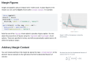
Margin Figures#

Figures that you create using code cells can be placed in the margin by using the column: margin code cell option. If the code produces more than one figure, each of the figures will be placed in the margin.

 1
 2
 3
 4
 5
 6
 7
 8
 9
10
11
12
13
14
15

```{r}
#| label: fig-mtcars
#| fig-cap: "MPG vs horsepower, colored by transmission."
#| column: margin

library(ggplot2)
mtcars2 <- mtcars
mtcars2$am <- factor(
  mtcars$am, labels = c('automatic', 'manual')
)
ggplot(mtcars2, aes(hp, mpg, color = am)) +
  geom_point() +
  geom_smooth(formula = y ~ x, method = "loess") +
  theme(legend.position = 'bottom')
```

Margin Tables#

You an also place tables in the margin of your document by specifying column: margin.

1
2
3
4
5
6
7

```{r}
#| column: margin

knitr::kable(
  mtcars[1:3, 1:3]
)
```

Other Content#

You can also place content in the margin by targeting the margin column using a div with the .column-margin class. For example:

1
2
3
4
5

::: {.column-margin}
We know from *the first fundamental theorem of calculus* that for $x$ in $[a, b]$:

$$\frac{d}{dx}\left( \int_{a}^{x} f(u)\,du\right)=f(x).$$
:::

We know from the first fundamental theorem of calculus that for $x$ in $[a, b]$:

$$\frac{d}{dx}\left( \int_{a}^{x} f(u),du\right)=f(x).$$

Margin References#

Footnotes and the bibliography typically appear at the end of the document, but you can choose to have them placed in the margin by setting the following option[^1] in the document front matter:

1
2
3
4

---
reference-location: margin
citation-location: margin
---

With these options set, footnotes and citations will (respectively) be automatically be placed in the margin of the document rather than the bottom of the page. As an example, when I cite Xie et al. (2018), the citation bibliography entry itself will now appear in the margin.

Asides#

Asides allow you to place content aside from the content it is placed in. Asides look like footnotes, but do not include the footnote mark (the superscript number). This is a span that has the class aside which places it in the margin without a footnote number.

1

[This is a span that has the class aside which places it in the margin without a footnote number.]{.aside}

Margin Captions#

For figures and tables, you may leave the content in the body of the document while placing the caption in the margin of the document. Using cap-location: margin in a code cell or document front matter to control this. For example:

 1
 2
 3
 4
 5
 6
 7
 8
 9
10
11
12
13
14
15

```{r}
#| label: fig-cap-margin
#| fig-cap: "MPG vs horsepower, colored by transmission."
#| cap-location: margin

library(ggplot2)
mtcars2 <- mtcars
mtcars2$am <- factor(
  mtcars$am, labels = c('automatic', 'manual')
)
ggplot(mtcars2, aes(hp, mpg, color = am)) +
  geom_point() +
  geom_smooth(formula = y ~ x, method = "loess") +
  theme(legend.position = 'bottom')
```

References#

Xie, Yihui, J. J. Allaire, and Garrett Grolemund. 2018. R Markdown: The Definitive Guide. Chapman; Hall/CRC. https://bookdown.org/yihui/rmarkdown .