Great Tables: The Polars DataFrame Styler of Your Dreams

Analyzing data with polars is a no-brainer in python. It provides an intuitive, expressive interface to data. When it comes to reports, it’s trivial to plug polars into plotting libraries like seaborn, plotly, and plotnine.

However, there are fewer options for styling tables for presentation. You could convert from polars to pandas, and use the built-in pandas DataFrame styler , but this has one major limitation: you can’t use polars expressions.

As it turns out, polars expressions make styling tables very straightforward. The same polars code that you would use to select or filter combines with Great Tables to highlight, circle, or bolden text.

In this post, I’ll show how Great Tables uses polars expressions to make delightful tables, like the one below.

 1
 2
 3
 4
 5
 6
 7
 8
 9
10
11
12
13
14
15
16
17
18
19
20
21
22
23
24
25
26
27
28
29
30
31
32
33
34
35
36
37
38
39
40
41
42
43
44
45
46
47
48
49
50

import polars as pl
import polars.selectors as cs

from great_tables import GT, md, html, style, loc
from great_tables.data import airquality

airquality_mini = airquality.head(10).assign(Year = 1973)
pl_airquality = pl.DataFrame(airquality_mini).select(
    "Year", "Month", "Day", "Ozone", "Solar_R", "Wind", "Temp"
)
gt_air = GT(pl_airquality)

(
    gt_air

    # Table header ----
    .tab_header(
        title = "New York Air Quality Measurements",
        subtitle = "Daily measurements in New York City (May 1-10, 1973)"
    )

    # Table column spanners ----
    .tab_spanner(
        label = "Time",
        columns = ["Year", "Month", "Day"]
    )
    .tab_spanner(
        label = "Measurement",
        columns = ["Ozone", "Solar_R", "Wind", "Temp"]
    )
    .cols_label(
        Ozone = html("Ozone,<br>ppbV"),
        Solar_R = html("Solar R.,<br>cal/m<sup>2</sup>"),
        Wind = html("Wind,<br>mph"),
        Temp = html("Temp,<br>&deg;F")
    )

    # Table styles ----
    .tab_style(
        style.fill("lightyellow"),
        loc.body(
            columns = cs.all(),
            rows = pl.col("Wind") == pl.col("Wind").max()
        )
    )
    .tab_style(
        style.text(weight = "bold"),
        loc.body("Wind", pl.col("Wind") == pl.col("Wind").max())
    )
)

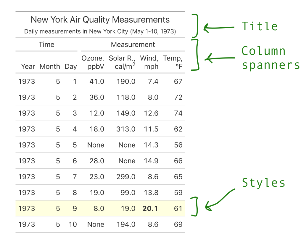
The parts of a presentation-ready table#

Our example table customized three main parts:

• Title and subtitle: User friendly titles and subtitles, describing the data.
• Column spanners: Group related columns together with a custom label.
• Styles: Highlight rows, columns, or individual cells of data.

This is marked below.

Let’s walk through each piece in order to produce the table below.

Creating GT object#

First, we’ll import the necessary libraries, and do a tiny bit of data processing.

 1
 2
 3
 4
 5
 6
 7
 8
 9
10
11
12
13

import polars as pl
import polars.selectors as cs

from great_tables import GT
from great_tables.data import airquality

# Note that we'll use the first 5 rows as we build up our code
airquality_mini = airquality.head(5).assign(Year = 1973)
pl_airquality = pl.DataFrame(airquality_mini).select(
    "Year", "Month", "Day", "Ozone", "Solar_R", "Wind", "Temp"
)

pl_airquality

The default polars output above is really helpful for data analysis! By passing it to the GT constructor, we can start getting it ready for presentation.

1
2
3

gt_air = GT(pl_airquality)

gt_air

In the next section I’ll show setting a title, and then go on to more exciting stuff like styling the body and creating column spanners.

Set title and subtitle#

The simplest method in gt is GT.tab_header(), which lets you add a title and subtitle.

1
2
3
4
5
6
7
8
9

(
    gt_air

    # Table header ----
    .tab_header(
        title = "New York Air Quality Measurements",
        subtitle = "Daily measurements in New York City (May 1-10, 1973)"
    )
)

Just like with plots, tables need titles so people know what they’re about!

Set body styles#

The .tab_style() method sets styles—like fill color, or text properties—on different parts of the table. Let’s use it twice with a polars expression. First to highlight the row corresponding to the max Wind value, and then to bold that value.

 1
 2
 3
 4
 5
 6
 7
 8
 9
10
11
12
13
14
15
16
17
18
19
20

from great_tables import style, loc

is_max_wind = pl.col("Wind") == pl.col("Wind").max()

(
    gt_air

    # Table styles ----
    .tab_style(
        style.fill("lightyellow"),
        loc.body(
            columns = cs.all(),
            rows = is_max_wind
        )
    )
    .tab_style(
        style.text(weight = "bold"),
        loc.body("Wind", is_max_wind)
    )
)

Note two important pieces:

• Functions like style.fill() indicate what style to set.
• Functions like loc.body() indicate where to apply the style. Its columns= and rows= parameters let you target specific parts of the table body (using polars expressions).

Currently, Great Tables only supports styling the table body. In the (very near) future, other loc.* functions will allow styling other parts of the table (e.g. the title, column labels, etc..).

For more details on styles, see Styling the Table Body in the Getting Started guide.

Set column spanners#

The last piece to set in the table is the column spanners, which are made up of two things:

• Labels describing groups of columns (e.g. Time, Measurement).
• More readable labels for columns themselves.

Use GT.tab_spanner() to set labels on groups of columns.

 1
 2
 3
 4
 5
 6
 7
 8
 9
10
11
12
13
14
15
16
17

time_cols = ["Year", "Month", "Day"]

gt_with_spanners = (
    gt_air

    # Table column spanners ----
    .tab_spanner(
        label="Time",
        columns=time_cols
    )
    .tab_spanner(
        label="Measurement",
        columns=cs.exclude(time_cols)
    )
)

gt_with_spanners

Notice that there are now labels for “Time” and “Measurement” sitting above the column names. This is useful for emphasizing columns that share something in common.

Use GT.cols_labels() with html() to create human-friendly labels (e.g. convert things like cal_m_2 to cal/m2).

 1
 2
 3
 4
 5
 6
 7
 8
 9
10
11

from great_tables import html

(
    gt_with_spanners
    .cols_label(
        Ozone = html("Ozone,<br>ppbV"),
        Solar_R = html("Solar R.,<br>cal/m<sup>2</sup>"),
        Wind = html("Wind,<br>mph"),
        Temp = html("Temp,<br>&deg;F")
    )
)

This is helpful because labels are often in a funky format (e.g. cal_m_2) because they’re easier to work with programmatically, so need to be cleaned up for presentation.

See the Column Labels page of the guide for more details.

Putting it all together#

Finally, we’ll combine everything from the sections above into a single block of code, and use a few more rows of data.

 1
 2
 3
 4
 5
 6
 7
 8
 9
10
11
12
13
14
15
16
17
18
19
20
21
22
23
24
25
26
27
28
29
30
31
32
33
34
35
36
37
38
39
40
41
42
43
44
45
46
47
48
49
50

import polars as pl
import polars.selectors as cs

from great_tables import GT, md, html, style, loc
from great_tables.data import airquality

airquality_mini = airquality.head(10).assign(Year = 1973)
pl_airquality = pl.DataFrame(airquality_mini).select(
    "Year", "Month", "Day", "Ozone", "Solar_R", "Wind", "Temp"
)
gt_air = GT(pl_airquality)

(
    gt_air

    # Table header ----
    .tab_header(
        title = "New York Air Quality Measurements",
        subtitle = "Daily measurements in New York City (May 1-10, 1973)"
    )

    # Table column spanners ----
    .tab_spanner(
        label = "Time",
        columns = ["Year", "Month", "Day"]
    )
    .tab_spanner(
        label = "Measurement",
        columns = ["Ozone", "Solar_R", "Wind", "Temp"]
    )
    .cols_label(
        Ozone = html("Ozone,<br>ppbV"),
        Solar_R = html("Solar R.,<br>cal/m<sup>2</sup>"),
        Wind = html("Wind,<br>mph"),
        Temp = html("Temp,<br>&deg;F")
    )

    # Table styles ----
    .tab_style(
        style.fill("lightyellow"),
        loc.body(
            columns = cs.all(),
            rows = pl.col("Wind") == pl.col("Wind").max()
        )
    )
    .tab_style(
        style.text(weight = "bold"),
        loc.body("Wind", pl.col("Wind") == pl.col("Wind").max())
    )
)

Not too bad!

Table styling is a surprisingly deep topic, and we’ve only scratched the surface on what Great Tables can do. A big one not covered here is the many column formatting methods , like GT.fmt_currency().

Thoughtfully styled tables tell viewers that you care as much about communicating the table, as much as the data wrangling behind it. Working with polars has been an absolute dream, and we’re excited to explore different ways it and Great Tables make for easy table styling!