The need to segment images arises in various sciences and their applications, many of which are vital to human (and animal) life. In this introductory post, we train a U-Net to mark lesioned regions on MRI brain scans
True, sometimes it’s vital to distinguish between different kinds of objects. Is that a car speeding towards me, in which case I’d better jump out of the way? Or is it a huge Doberman (in which case I’d probably do the same)? Often in real life though, instead of coarse-grained classification, what is needed is fine-grained segmentation.
Zooming in on images, we’re not looking for a single label; instead, we want to classify every pixel according to some criterion:
In medicine, we may want to distinguish between different cell types, or identify tumors.
In various earth sciences, satellite data are used to segment terrestrial surfaces.
To enable use of custom backgrounds, video-conferencing software has to be able to tell foreground from background.
Image segmentation is a form of supervised learning: Some kind of ground truth is needed. Here, it comes in form of a mask – an image, of spatial resolution identical to that of the input data, that designates the true class for every pixel. Accordingly, classification loss is calculated pixel-wise; losses are then summed up to yield an aggregate to be used in optimization.
The “canonical” architecture for image segmentation is U-Net (around since 2015).
Here is the prototypical U-Net, as depicted in the original Rönneberger et al. paper (Ronneberger et al. 2015).
Of this architecture, numerous variants exist. You could use different layer sizes, activations, ways to achieve downsizing and upsizing, and more. However, there is one defining characteristic: the U-shape, stabilized by the “bridges” crossing over horizontally at all levels.
The original U-Net, as depicted in Ronnerberger et al. (2015).
In a nutshell, the left-hand side of the U resembles the convolutional architectures used in image classification. It successively reduces spatial resolution. At the same time, another dimension – the channels dimension – is used to build up a hierarchy of features, ranging from very basic to very specialized.
Unlike in classification, however, the output should have the same spatial resolution as the input. Thus, we need to upsize again – this is taken care of by the right-hand side of the U. But, how are we going to arrive at a good per-pixel classification, now that so much spatial information has been lost?
This is what the “bridges” are for: At each level, the input to an upsampling layer is a concatenation of the previous layer’s output – which went through the whole compression/decompression routine – and some preserved intermediate representation from the downsizing phase. In this way, a U-Net architecture combines attention to detail with feature extraction.
With U-Net, domain applicability is as broad as the architecture is flexible. Here, we want to detect abnormalities in brain scans. The dataset, used in Buda et al. (2019), contains MRI images together with manually created FLAIR
abnormality segmentation masks. It is available on Kaggle
.
Nicely, the paper is accompanied by a GitHub repository
. Below, we closely follow (though not exactly replicate) the authors’ preprocessing and data augmentation code.
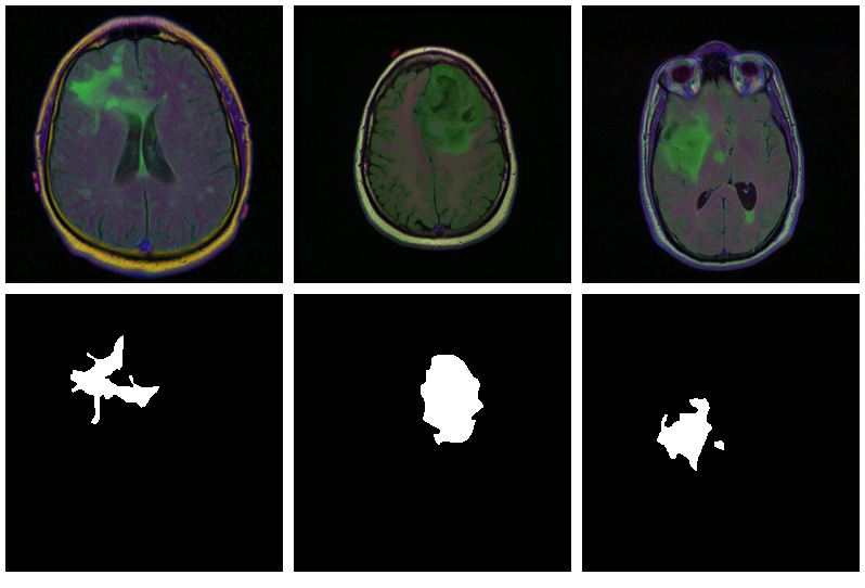
As is often the case in medical imaging, there is notable class imbalance in the data. For every patient, sections have been taken at multiple positions. (Number of sections per patient varies.) Most sections do not exhibit any lesions; the corresponding masks are colored black everywhere.
Here are three examples where the masks do indicate abnormalities:
Let’s see if we can build a U-Net that generates such masks for us.
# deep learning (incl. dependencies)library(torch)library(torchvision)# data wranglinglibrary(tidyverse)library(zeallot)# image processing and visualizationlibrary(magick)library(cowplot)# dataset loading library(pins)library(zip)torch_manual_seed(777)set.seed(777)# use your own kaggle.json herepins::board_register_kaggle(token="~/kaggle.json")files<-pins::pin_get("mateuszbuda/lgg-mri-segmentation",board="kaggle",extract=FALSE)
The dataset is not that big – it includes scans from 110 different patients – so we’ll have to do with just a training and a validation set. (Don’t do this in real life, as you’ll inevitably end up fine-tuning on the latter.)
 1
 2
 3
 4
 5
 6
 7
 8
 9
10
11
12
13
14
15
train_dir<-"data/mri_train"valid_dir<-"data/mri_valid"if(dir.exists(train_dir))unlink(train_dir,recursive=TRUE,force=TRUE)if(dir.exists(valid_dir))unlink(valid_dir,recursive=TRUE,force=TRUE)zip::unzip(files,exdir="data")file.rename("data/kaggle_3m",train_dir)# this is a duplicate, again containing kaggle_3m (evidently a packaging error on Kaggle)# we just remove itunlink("data/lgg-mri-segmentation",recursive=TRUE)dir.create(valid_dir)
Of those 110 patients, we keep 30 for validation. Some more file manipulations, and we’re set up with a nice hierarchical structure, with train_dir and valid_dir holding their per-patient sub-directories, respectively.
Like every torch dataset, this one has initialize() and .getitem() methods. initialize() creates an inventory of scan and mask file names, to be used by .getitem() when it actually reads those files. In contrast to what we’ve seen in previous posts, though , .getitem() does not simply return input-target pairs in order. Instead, whenever the parameter random_sampling is true, it will perform weighted sampling, preferring items with sizable lesions. This option will be used for the training set, to counter the class imbalance mentioned above.
The other way training and validation sets will differ is use of data augmentation. Training images/masks may be flipped, re-sized, and rotated; probabilities and amounts are configurable.
An instance of brainseg_dataset encapsulates all this functionality:
With torch, it is straightforward to inspect what happens when you change augmentation-related parameters. We just pick a pair from the validation set, which has not had any augmentation applied as yet, and call valid_ds$<augmentation_func()> directly. Just for fun, let’s use more “extreme” parameters here than we do in actual training. (Actual training uses the settings from Mateusz’ GitHub repository, which we assume have been carefully chosen for optimal performance.1)
Our model nicely illustrates the kind of modular code that comes “naturally” with torch. We approach things top-down, starting with the U-Net container itself.
unet takes care of the global composition – how far “down” do we go, shrinking the image while incrementing the number of filters, and then how do we go “up” again?
Importantly, it is also in the system’s memory. In forward(), it keeps track of layer outputs seen going “down”, to be added back in going “up”.
unet delegates to two containers just below it in the hierarchy: down_block and up_block. While down_block is “just” there for aesthetic reasons (it immediately delegates to its own workhorse, conv_block), in up_block we see the U-Net “bridges” in action.
Optimization uses stochastic gradient descent (SGD), together with the one-cycle learning rate scheduler introduced in the context of image classification with torch
.
The training loop then follows the usual scheme. One thing to note: Every epoch, we save the model (using torch_save()), so we can later pick the best one, should performance have degraded thereafter.
Now, since we don’t have a separate test set, we already know the average out-of-sample metrics; but in the end, what we care about are the generated masks. Let’s view some, displaying ground truth and MRI scans for comparison.
# without random sampling, we'd mainly see lesion-free patcheseval_ds<-brainseg_dataset(valid_dir,augmentation_params=NULL,random_sampling=TRUE)eval_dl<-dataloader(eval_ds,batch_size=8)batch<-eval_dl%>%dataloader_make_iter()%>%dataloader_next()par(mfcol=c(3,8),mar=c(0,1,0,1))for(iin1:8){img<-batch[[1]][i,..,drop=FALSE]inferred_mask<-model(img$to(device=device))true_mask<-batch[[2]][i,..,drop=FALSE]$to(device=device)bce<-nnf_binary_cross_entropy(inferred_mask,true_mask)$to(device="cpu")%>%as.numeric()dc<-calc_dice_loss(inferred_mask,true_mask)$to(device="cpu")%>%as.numeric()cat(sprintf("\nSample %d, bce: %3f, dice: %3f\n",i,bce,dc))inferred_mask<-inferred_mask$to(device="cpu")%>%as.array()%>%.[1,1,,]inferred_mask<-ifelse(inferred_mask>0.5,1,0)img[1,1,,]%>%as.array()%>%as.raster()%>%plot()true_mask$to(device="cpu")[1,1,,]%>%as.array()%>%as.raster()%>%plot()inferred_mask%>%as.raster()%>%plot()}
We also print the individual cross entropy and dice losses; relating those to the generated masks might yield useful information for model tuning.
This has been our most complex torch post so far; however, we hope you’ve found the time well spent. For one, among applications of deep learning, medical image segmentation stands out as highly societally useful. Secondly, U-Net-like architectures are employed in many other areas. And finally, we once more saw torch’s flexibility and intuitive behavior in action.
Thanks for reading!
Buda, Mateusz, Ashirbani Saha, and Maciej A. Mazurowski. 2019. “Association of Genomic Subtypes of Lower-Grade Gliomas with Shape Features Automatically Extracted by a Deep Learning Algorithm.” Computers in Biology and Medicine 109: 218–25. https://doi.org/https://doi.org/10.1016/j.compbiomed.2019.05.002
.
Ronneberger, Olaf, Philipp Fischer, and Thomas Brox. 2015. “U-Net: Convolutional Networks for Biomedical Image Segmentation.” CoRR abs/1505.04597. http://arxiv.org/abs/1505.04597
.
Yes, we did a few experiments, confirming that more augmentation isn’t better … what did I say about inevitably ending up doing optimization on the validation set …? ↩︎
Hugging Face rapidly became a very popular platform to build, share and collaborate on deep learning applications. We have worked on integrating the torch for R ecosystem with Hugging Face tools, allowing users to load and execute language models from their platform.
LoRA (Low Rank Adaptation) is a new technique for fine-tuning deep learning models that works by reducing the number of trainable parameters and enables efficient task switching. In this blog post we will talk about the key ideas behind LoRA in a very minimal torch example.
Implementing a language model from scratch is, arguably, the best way to develop an accurate idea of how its engine works. Here, we use torch to code GPT-2, the immediate successor to the original GPT. In the end, you’ll dispose of an R-native model that can make direct use of Hugging Face’s pre-trained GPT-2 model weights.
Stay Connected
Get the latest updates on Posit open source projects and insights from our community.

.")