About two weeks ago, we introduced TensorFlow Probability (TFP) , showing how to create and sample from distributions and put them to use in a Variational Autoencoder (VAE) that learns its prior. Today, we move on to a different specimen in the VAE model zoo: the Vector Quantised Variational Autoencoder (VQ-VAE) described in Neural Discrete Representation Learning (Oord et al. 2017). This model differs from most VAEs in that its approximate posterior is not continuous, but discrete - hence the “quantised” in the article’s title. We’ll quickly look at what this means, and then dive directly into the code, combining Keras layers, eager execution, and TFP.

Discrete codes#

Many phenomena are best thought of, and modeled, as discrete. This holds for phonemes and lexemes in language, higher-level structures in images (think objects instead of pixels),and tasks that necessitate reasoning and planning. The latent code used in most VAEs, however, is continuous - usually it’s a multivariate Gaussian. Continuous-space VAEs have been found very successful in reconstructing their input, but often they suffer from something called posterior collapse: The decoder is so powerful that it may create realistic output given just any input. This means there is no incentive to learn an expressive latent space.

In VQ-VAE, however, each input sample gets mapped deterministically to one of a set of embedding vectors ¹. Together, these embedding vectors constitute the prior for the latent space. As such, an embedding vector contains a lot more information than a mean and a variance, and thus, is much harder to ignore by the decoder.

The question then is: Where is that magical hat, for us to pull out meaningful embeddings?

Learning a discrete embedding space#

From the above conceptual description, we now have two questions to answer. First, by what mechanism do we assign input samples (that went through the encoder) to appropriate embedding vectors? And second: How can we learn embedding vectors that actually are useful representations - that when fed to a decoder, will result in entities perceived as belonging to the same species?

As regards assignment, a tensor emitted from the encoder is simply mapped to its nearest neighbor in embedding space, using Euclidean distance. The embedding vectors are then updated using exponential moving averages ². As we’ll see soon, this means that they are actually not being learned using gradient descent - a feature worth pointing out as we don’t come across it every day in deep learning.

Concretely, how then should the loss function and training process look? This will probably easiest be seen in code.

Coding the VQ-VAE#

The complete code for this example, including utilities for model saving and image visualization, is available on github as part of the Keras examples. Order of presentation here may differ from actual execution order for expository purposes, so please to actually run the code consider making use of the example on github.

Setup and data loading#

As in all our prior posts on VAEs, we use eager execution, which presupposes the TensorFlow implementation of Keras.

 1
 2
 3
 4
 5
 6
 7
 8
 9
10
11
12
13
14


library(keras)
use_implementation("tensorflow")
library(tensorflow)
tfe_enable_eager_execution(device_policy = "silent")

tfp <- import("tensorflow_probability")
tfd <- tfp$distributions

library(tfdatasets)
library(dplyr)
library(glue)
# used for set_defaults; please get the development version:
# devtools::install_github("thomasp85/curry")
library(curry) 

As in our previous post on doing VAE with TFP, we’ll use Kuzushiji-MNIST (Clanuwat et al. 2018) as input. Now is the time to look at what we ended up generating that time and place your bet: How will that compare against the discrete latent space of VQ-VAE?

 1
 2
 3
 4
 5
 6
 7
 8
 9
10
11
12
13
14
15
16
17
18
19
20


np <- import("numpy")
 
kuzushiji <- np$load("kmnist-train-imgs.npz")
kuzushiji <- kuzushiji$get("arr_0")

train_images <- kuzushiji %>%
  k_expand_dims() %>%
  k_cast(dtype = "float32")

train_images <- train_images %>% `/`(255)

buffer_size <- 60000
batch_size <- 64
num_examples_to_generate <- batch_size

batches_per_epoch <- buffer_size / batch_size

train_dataset <- tensor_slices_dataset(train_images) %>%
  dataset_shuffle(buffer_size) %>%
  dataset_batch(batch_size, drop_remainder = TRUE)

Hyperparameters#

In addition to the “usual” hyperparameters we have in deep learning, the VQ-VAE infrastructure introduces a few model-specific ones. First of all, the embedding space is of dimensionality number of embedding vectors times embedding vector size:

1
2
3
4


# number of embedding vectors
num_codes <- 64L
# dimensionality of the embedding vectors
code_size <- 16L

The latent space in our example will be of size one, that is, we have a single embedding vector representing the latent code for each input sample. This will be fine for our dataset, but it should be noted that van den Oord et al. used far higher-dimensional latent spaces on e.g. ImageNet and Cifar-10 ³.

1

latent_size <- 1

Encoder model#

The encoder uses convolutional layers to extract image features. Its output is a 3-d tensor of shape batchsize * 1 * code_size.

1
2
3


activation <- "elu"
# modularizing the code just a little bit
default_conv <- set_defaults(layer_conv_2d, list(padding = "same", activation = activation))

 1
 2
 3
 4
 5
 6
 7
 8
 9
10
11
12
13
14
15
16
17
18
19
20
21
22
23
24
25
26
27
28
29
30
31
32
33
34
35
36
37


base_depth <- 32

encoder_model <- function(name = NULL,
                          code_size) {
  
  keras_model_custom(name = name, function(self) {
    
    self$conv1 <- default_conv(filters = base_depth, kernel_size = 5)
    self$conv2 <- default_conv(filters = base_depth, kernel_size = 5, strides = 2)
    self$conv3 <- default_conv(filters = 2 * base_depth, kernel_size = 5)
    self$conv4 <- default_conv(filters = 2 * base_depth, kernel_size = 5, strides = 2)
    self$conv5 <- default_conv(filters = 4 * latent_size, kernel_size = 7, padding = "valid")
    self$flatten <- layer_flatten()
    self$dense <- layer_dense(units = latent_size * code_size)
    self$reshape <- layer_reshape(target_shape = c(latent_size, code_size))
    
    function (x, mask = NULL) {
      x %>% 
        # output shape:  7 28 28 32 
        self$conv1() %>% 
        # output shape:  7 14 14 32 
        self$conv2() %>% 
        # output shape:  7 14 14 64 
        self$conv3() %>% 
        # output shape:  7 7 7 64 
        self$conv4() %>% 
        # output shape:  7 1 1 4 
        self$conv5() %>% 
        # output shape:  7 4 
        self$flatten() %>% 
        # output shape:  7 16 
        self$dense() %>% 
        # output shape:  7 1 16
        self$reshape()
    }
  })
}

As always, let’s make use of the fact that we’re using eager execution, and see a few example outputs.

1
2
3
4
5
6


iter <- make_iterator_one_shot(train_dataset)
batch <-  iterator_get_next(iter)

encoder <- encoder_model(code_size = code_size)
encoded  <- encoder(batch)
encoded

tf.Tensor(
[[[ 0.00516277 -0.00746826  0.0268365  ... -0.012577   -0.07752544
   -0.02947626]]
...

 [[-0.04757921 -0.07282603 -0.06814402 ... -0.10861694 -0.01237121
    0.11455103]]], shape=(64, 1, 16), dtype=float32)

Now, each of these 16d vectors needs to be mapped to the embedding vector it is closest to. This mapping is taken care of by another model: vector_quantizer.

Vector quantizer model#

This is how we will instantiate the vector quantizer:

1

vector_quantizer <- vector_quantizer_model(num_codes = num_codes, code_size = code_size)

This model serves two purposes: First, it acts as a store for the embedding vectors. Second, it matches encoder output to available embeddings.

Here, the current state of embeddings is stored in codebook. ema_means and ema_count are for bookkeeping purposes only (note how they are set to be non-trainable). We’ll see them in use shortly.

 1
 2
 3
 4
 5
 6
 7
 8
 9
10
11
12
13
14
15
16
17
18
19
20
21
22
23
24
25
26
27
28
29


vector_quantizer_model <- function(name = NULL, num_codes, code_size) {
  
    keras_model_custom(name = name, function(self) {
      
      self$num_codes <- num_codes
      self$code_size <- code_size
      self$codebook <- tf$get_variable(
        "codebook",
        shape = c(num_codes, code_size), 
        dtype = tf$float32
        )
      self$ema_count <- tf$get_variable(
        name = "ema_count", shape = c(num_codes),
        initializer = tf$constant_initializer(0),
        trainable = FALSE
        )
      self$ema_means = tf$get_variable(
        name = "ema_means",
        initializer = self$codebook$initialized_value(),
        trainable = FALSE
        )
      
      function (x, mask = NULL) { 
        
        # to be filled in shortly ...
        
      }
    })
}

In addition to the actual embeddings, in its call method vector_quantizer holds the assignment logic. First, we compute the Euclidean distance of each encoding to the vectors in the codebook (tf$norm). We assign each encoding to the closest as by that distance embedding (tf$argmin) and one-hot-encode the assignments (tf$one_hot). Finally, we isolate the corresponding vector by masking out all others and summing up what’s left over (multiplication followed by tf$reduce_sum).

Regarding the axis argument used with many TensorFlow functions, please take into consideration that in contrast to their k_* siblings, raw TensorFlow (tf$*) functions expect axis numbering to be 0-based. We also have to add the L’s after the numbers to conform to TensorFlow’s datatype requirements.

 1
 2
 3
 4
 5
 6
 7
 8
 9
10
11
12
13
14
15
16
17
18
19
20
21
22
23
24
25
26
27
28
29
30
31
32
33


vector_quantizer_model <- function(name = NULL, num_codes, code_size) {
  
    keras_model_custom(name = name, function(self) {
      
      # here we have the above instance fields
      
      function (x, mask = NULL) {
    
        # shape: bs * 1 * num_codes
         distances <- tf$norm(
          tf$expand_dims(x, axis = 2L) -
            tf$reshape(self$codebook, 
                       c(1L, 1L, self$num_codes, self$code_size)),
                       axis = 3L 
        )
        
        # bs * 1
        assignments <- tf$argmin(distances, axis = 2L)
        
        # bs * 1 * num_codes
        one_hot_assignments <- tf$one_hot(assignments, depth = self$num_codes)
        
        # bs * 1 * code_size
        nearest_codebook_entries <- tf$reduce_sum(
          tf$expand_dims(
            one_hot_assignments, -1L) * 
            tf$reshape(self$codebook, c(1L, 1L, self$num_codes, self$code_size)),
                       axis = 2L 
                       )
        list(nearest_codebook_entries, one_hot_assignments)
      }
    })
  }

Now that we’ve seen how the codes are stored, let’s add functionality for updating them. As we said above, they are not learned via gradient descent. Instead, they are exponential moving averages, continually updated by whatever new “class member” they get assigned.

So here is a function update_ema that will take care of this.

update_ema uses TensorFlow moving_averages to

first, keep track of the number of currently assigned samples per code (updated_ema_count), and
second, compute and assign the current exponential moving average (updated_ema_means).

 1
 2
 3
 4
 5
 6
 7
 8
 9
10
11
12
13
14
15
16
17
18
19
20
21
22
23
24
25
26
27
28
29
30
31
32
33
34


moving_averages <- tf$python$training$moving_averages

# decay to use in computing exponential moving average
decay <- 0.99

update_ema <- function(
  vector_quantizer,
  one_hot_assignments,
  codes,
  decay) {
 
  updated_ema_count <- moving_averages$assign_moving_average(
    vector_quantizer$ema_count,
    tf$reduce_sum(one_hot_assignments, axis = c(0L, 1L)),
    decay,
    zero_debias = FALSE
  )

  updated_ema_means <- moving_averages$assign_moving_average(
    vector_quantizer$ema_means,
    # selects all assigned values (masking out the others) and sums them up over the batch
    # (will be divided by count later, so we get an average)
    tf$reduce_sum(
      tf$expand_dims(codes, 2L) *
        tf$expand_dims(one_hot_assignments, 3L), axis = c(0L, 1L)),
    decay,
    zero_debias = FALSE
  )

  updated_ema_count <- updated_ema_count + 1e-5
  updated_ema_means <-  updated_ema_means / tf$expand_dims(updated_ema_count, axis = -1L)
  
  tf$assign(vector_quantizer$codebook, updated_ema_means)
}

Before we look at the training loop, let’s quickly complete the scene adding in the last actor, the decoder.

Decoder model#

The decoder is pretty standard, performing a series of deconvolutions and finally, returning a probability for each image pixel.

 1
 2
 3
 4
 5
 6
 7
 8
 9
10
11
12
13
14
15
16
17
18
19
20
21
22
23
24
25
26
27
28
29
30
31
32
33
34
35
36
37
38
39
40
41
42
43
44
45
46
47
48
49
50
51
52
53
54
55
56
57
58
59
60
61
62
63
64
65
66
67
68


default_deconv <- set_defaults(
  layer_conv_2d_transpose,
  list(padding = "same", activation = activation)
)

decoder_model <- function(name = NULL,
                          input_size,
                          output_shape) {
  
  keras_model_custom(name = name, function(self) {
    
    self$reshape1 <- layer_reshape(target_shape = c(1, 1, input_size))
    self$deconv1 <-
      default_deconv(
        filters = 2 * base_depth,
        kernel_size = 7,
        padding = "valid"
      )
    self$deconv2 <-
      default_deconv(filters = 2 * base_depth, kernel_size = 5)
    self$deconv3 <-
      default_deconv(
        filters = 2 * base_depth,
        kernel_size = 5,
        strides = 2
      )
    self$deconv4 <-
      default_deconv(filters = base_depth, kernel_size = 5)
    self$deconv5 <-
      default_deconv(filters = base_depth,
                     kernel_size = 5,
                     strides = 2)
    self$deconv6 <-
      default_deconv(filters = base_depth, kernel_size = 5)
    self$conv1 <-
      default_conv(filters = output_shape[3],
                   kernel_size = 5,
                   activation = "linear")
    
    function (x, mask = NULL) {
      
      x <- x %>%
        # output shape:  7 1 1 16
        self$reshape1() %>%
        # output shape:  7 7 7 64
        self$deconv1() %>%
        # output shape:  7 7 7 64
        self$deconv2() %>%
        # output shape:  7 14 14 64
        self$deconv3() %>%
        # output shape:  7 14 14 32
        self$deconv4() %>%
        # output shape:  7 28 28 32
        self$deconv5() %>%
        # output shape:  7 28 28 32
        self$deconv6() %>%
        # output shape:  7 28 28 1
        self$conv1()
      
      tfd$Independent(tfd$Bernoulli(logits = x),
                      reinterpreted_batch_ndims = length(output_shape))
    }
  })
}

input_shape <- c(28, 28, 1)
decoder <- decoder_model(input_size = latent_size * code_size,
                         output_shape = input_shape)

Now we’re ready to train. One thing we haven’t really talked about yet is the cost function: Given the differences in architecture (compared to standard VAEs), will the losses still look as expected (the usual add-up of reconstruction loss and KL divergence)? We’ll see that in a second.

Training loop#

Here’s the optimizer we’ll use. Losses will be calculated inline.

1

optimizer <- tf$train$AdamOptimizer(learning_rate = learning_rate)

The training loop, as usual, is a loop over epochs, where each iteration is a loop over batches obtained from the dataset. For each batch, we have a forward pass, recorded by a gradientTape, based on which we calculate the loss. The tape will then determine the gradients of all trainable weights throughout the model, and the optimizer will use those gradients to update the weights.

So far, all of this conforms to a scheme we’ve oftentimes seen before. One point to note though: In this same loop, we also call update_ema to recalculate the moving averages, as those are not operated on during backprop. Here is the essential functionality: ⁴

 1
 2
 3
 4
 5
 6
 7
 8
 9
10
11
12
13
14
15
16
17
18
19
20
21
22
23
24
25
26
27
28
29
30
31
32
33
34
35
36
37
38
39


num_epochs <- 20

for (epoch in seq_len(num_epochs)) {
  
  iter <- make_iterator_one_shot(train_dataset)
  
  until_out_of_range({
    
    x <-  iterator_get_next(iter)
    with(tf$GradientTape(persistent = TRUE) %as% tape, {
      
      # do forward pass
      # calculate losses
      
    })
    
    encoder_gradients <- tape$gradient(loss, encoder$variables)
    decoder_gradients <- tape$gradient(loss, decoder$variables)
    
    optimizer$apply_gradients(purrr::transpose(list(
      encoder_gradients, encoder$variables
    )),
    global_step = tf$train$get_or_create_global_step())
    
    optimizer$apply_gradients(purrr::transpose(list(
      decoder_gradients, decoder$variables
    )),
    global_step = tf$train$get_or_create_global_step())
    
    update_ema(vector_quantizer,
               one_hot_assignments,
               codes,
               decay)

    # periodically display some generated images
    # see code on github 
    # visualize_images("kuzushiji", epoch, reconstructed_images, random_images)
  })
}

Now, for the actual action. Inside the context of the gradient tape, we first determine which encoded input sample gets assigned to which embedding vector.

1
2


codes <- encoder(x)
c(nearest_codebook_entries, one_hot_assignments) %<-% vector_quantizer(codes)

Now, for this assignment operation there is no gradient. Instead what we can do is pass the gradients from decoder input straight through to encoder output. Here tf$stop_gradient exempts nearest_codebook_entries from the chain of gradients, so encoder and decoder are linked by codes:

1
2


codes_straight_through <- codes + tf$stop_gradient(nearest_codebook_entries - codes)
decoder_distribution <- decoder(codes_straight_through)

In sum, backprop will take care of the decoder’s as well as the encoder’s weights, whereas the latent embeddings are updated using moving averages, as we’ve seen already.

Now we’re ready to tackle the losses. There are three components:

First, the reconstruction loss, which is just the log probability of the actual input under the distribution learned by the decoder.

1

reconstruction_loss <- -tf$reduce_mean(decoder_distribution$log_prob(x))

Second, we have the commitment loss, defined as the mean squared deviation of the encoded input samples from the nearest neighbors they’ve been assigned to: We want the network to “commit” to a concise set of latent codes!

1

commitment_loss <- tf$reduce_mean(tf$square(codes - tf$stop_gradient(nearest_codebook_entries)))

Finally, we have the usual KL diverge to a prior. As, a priori, all assignments are equally probable, this component of the loss is constant and can oftentimes be dispensed of. We’re adding it here mainly for illustrative purposes.

1
2
3
4
5
6
7


prior_dist <- tfd$Multinomial(
  total_count = 1,
  logits = tf$zeros(c(latent_size, num_codes))
  )
prior_loss <- -tf$reduce_mean(
  tf$reduce_sum(prior_dist$log_prob(one_hot_assignments), 1L)
  )

Summing up all three components, we arrive at the overall loss ⁵:

1
2


beta <- 0.25
loss <- reconstruction_loss + beta * commitment_loss + prior_loss

Before we look at the results, let’s see what happens inside gradientTape at a single glance:

 1
 2
 3
 4
 5
 6
 7
 8
 9
10
11
12
13
14
15
16
17


with(tf$GradientTape(persistent = TRUE) %as% tape, {
      
  codes <- encoder(x)
  c(nearest_codebook_entries, one_hot_assignments) %<-% vector_quantizer(codes)
  codes_straight_through <- codes + tf$stop_gradient(nearest_codebook_entries - codes)
  decoder_distribution <- decoder(codes_straight_through)
      
  reconstruction_loss <- -tf$reduce_mean(decoder_distribution$log_prob(x))
  commitment_loss <- tf$reduce_mean(tf$square(codes - tf$stop_gradient(nearest_codebook_entries)))
  prior_dist <- tfd$Multinomial(
    total_count = 1,
    logits = tf$zeros(c(latent_size, num_codes))
  )
  prior_loss <- -tf$reduce_mean(tf$reduce_sum(prior_dist$log_prob(one_hot_assignments), 1L))
  
  loss <- reconstruction_loss + beta * commitment_loss + prior_loss
})

Results#

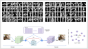
And here we go. This time, we can’t have the 2d “morphing view” one generally likes to display with VAEs (there just is no 2d latent space). Instead, the two images below are (1) letters generated from random input and (2) reconstructed actual letters, each saved after training for nine epochs.

Left: letters generated from random input. Right: reconstructed input letters.

Two things jump to the eye: First, the generated letters are significantly sharper than their continuous-prior counterparts (from the previous post). And second, would you have been able to tell the random image from the reconstruction image?

Conclusion#

At this point, we’ve hopefully convinced you of the power and effectiveness of this discrete-latents approach. However, you might secretly have hoped we’d apply this to more complex data, such as the elements of speech we mentioned in the introduction, or higher-resolution images as found in ImageNet. ⁶

The truth is that there’s a continuous tradeoff between the number of new and exciting techniques we can show, and the time we can spend on iterations to successfully apply these techniques to complex datasets. In the end it’s you, our readers, who will put these techniques to meaningful use on relevant, real world data.

Clanuwat, Tarin, Mikel Bober-Irizar, Asanobu Kitamoto, Alex Lamb, Kazuaki Yamamoto, and David Ha. 2018. “Deep Learning for Classical Japanese Literature.” December 3. https://arxiv.org/abs/cs.CV/1812.01718 .

Oord, Aaron van den, Oriol Vinyals, and Koray Kavukcuoglu. 2017. “Neural Discrete Representation Learning.” CoRR abs/1711.00937. http://arxiv.org/abs/1711.00937 .

Assuming a 1d latent space, that is. The authors actually used 1d, 2d and 3d spaces in their experiments. ↩︎
In the paper, the authors actually mention this as one of two ways to learn the prior, the other one being vector quantisation. ↩︎
To be specific, the authors indicate that they used a field of 32 x 32 latents for ImageNet, and 8 x 8 x 10 for CIFAR10. ↩︎
The code on github additionally contains functionality to display generated images, output the losses, and save checkpoints. ↩︎
Here beta is a scaling parameter found surprisingly unimportant by the paper authors. ↩︎
Although we have to say we find that Kuzushiji-MNIST beats MNIST by far, in complexity and aesthetics! ↩︎